Preface. Currently energy storage is accomplished with the 67% of fossil fuels (natural gas and coal) used to generate electricity, especially natural gas which can kick in within microseconds to make up for failing wind, or run all the time when there’s no wind or sun.

But the vast majority of states will never have to worry about energy storage because they have minimal wind, solar, or both. Currently just 9 states contribute 88% of solar generation, and 9 states generate 74% of wind power.  The dreams of most states going 100% renewable will always be a dream (Gattie 2019).

Solar power can’t possibly provide power year-round, it varies far too much (Smil, V. 2017. Power Density. MIT):

“Differences in monthly insolation averages depend on latitude and cloudiness: in Oslo the difference between January and June is 16-fold; in Riyadh it is only 2-fold.

As reflected by actual PV electricity generation, in 2012 the German output was 4 TWh in May and just 0.35 TWh in January, 11 times less, an order of magnitude disparity (BSW Solar 2013).

Average capacity factors correlate with total irradiance. in places where it is less than 150 W/m2 they will be below 12%, for the insolation between 150 and 200 W/m2 they will range up to 20%, and in the sunniest locations with irradiance in excess of 200 W/m2 they will be up to 25%. Actual performance data show that even in sunny Spain, most plants have capacity factors of less than 20%, and in cloudy temperate climates that indicator will dip below 10%. In addition, only about 85% of a PV panel’s DC rating will be transmitted to the grid as AC power”

Alice Friedemann   www.energyskeptic.com  author of “When Trucks Stop Running: Energy and the Future of Transportation”, 2015, Springer and “Crunch! Whole Grain Artisan Chips and Crackers”. Podcasts: Practical Prepping, KunstlerCast 253, KunstlerCast278, Peak Prosperity , XX2 report

***

Mulder, F. M. 2014. Implications of diurnal and seasonal variations in renewable energy generation for large scale energy storage. Journal of Renewable and Sustainable Energy. 14 pages.

Excerpts:

Large scale implementation of solar and wind powered renewable electricity generation will use up to continent sized connected electricity grids built to distribute the locally fluctuating power. Systematic power output variation will then become manifest since solar power has an evident diurnal period, but also surface winds—which are driven by surface temperatures—follow a diurnal periodic behavior lagging about 4 hours in time. On an ordinary day a strong diurnal varying renewable electricity generation results when combining wind and solar power on such continent sized grid. Comparison with possible demand patterns indicates that coping with such systematically varying generation will require large scale renewable energy storage and conversion for timescales and storage capacities of at least up to half a day. Seasonal timescales for versatile, high quality, generally applicable, energy conversion and storage are equally essential since the continent wide insolation varies by a factor ~3, e.g., in Europe and Northern Africa together. A first order model for estimating required energy storage and conversion magnitudes is presented, taking into account potential diurnal and seasonal energy demand and generation patterns.

The insolation (solar radiation power per square meter at the earth’s surface) is daily modulated between zero and a maximum that depends on the latitude on earth and the season (Figure 1). For instance in Edmonton in Canada, Delft in the Netherlands, and Astana in Kazachstan (~52 North), there is a factor of 6 between the insolation in mid-summer and mid-winter due to the reduced instantaneous light intensity and time of daylight as shown below:

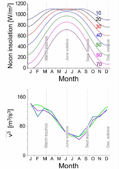
FIG. 1. Top: daily insolation at noon during the months of the year on the indicated northern latitudes. See also Fig. S1 in the supplementary material4 for the total daily insolation. Bottom: estimated average cubed windspeed v3 in the US for on shore (blue) and off shore (purple) locations (based on data from Ref. 5), and a simple sinusoidal approximation as in Eq. (2) (green).

In Mexico City, the Western Sahara and Nagpur in central India (~19.5 North), the factor between summer and winter reduces but still reaches a sizeable factor of about ~1.5. Thus in principle a factor of 6 to 1.5 difference per solar power collecting footprint between seasons occurs, next to the diurnal day and night fluctuations, and varying cloud covers. These seasonal and diurnal influences multiply with each other to obtain the total solar power. For a multi-grid connected surface area spanning Europe and Northern Africa this will mean on average a sizeable factor ~3–4 between summer and winter insolation, modulating the day and night diurnal variation on a seasonal scale.

Wind resources within a continent sized electricity grid depend on the instantaneous wind speeds averaged over the grid surface area. It is well known that the wind power is about two times stronger in winter than in summer on northern latitudes (Figure 1).

Within this seasonal timescale there is however also a diurnal periodicity of relevance. In meteorological literature a number of data studies are available of the near surface layer average wind speeds over extended surface area’s in Africa and the North Atlantic, and the US in which thousands of local weather stations have been taken into account. The general insight gained is that there is a diurnal variation in wind speeds with significant amplitude, where the peak in wind amplitudes occurs in the afternoon and the minimum 12 h earlier in the early morning.

For instance in Ref. 7, the instantaneous wind speed averaged over a ~800 X 1000 km2 surface area on an ordinary day could be 4–5 m/s while the minimum could be 2 m/s (Figure 2). The wind speed amplitude has such diurnal pattern because it is driven by the surface temperature, i.e., the solar radiation heating the surface and atmosphere above it drives the observed wind speeds.

Since the kinetic energy contained in flowing air scales with the third power of the wind speed a factor 2 in wind speed amplitude means a factor 8 in recoverable energy in wind turbines.

Offshore: The wind patterns and diurnal variation in those is determined by the significant differential heating of the water and land area. During the day the land warms relatively fast due to solar light absorption and the cooler and denser air from the adjacent ocean flows over the land.13 At night the land cooling takes place by the continued emission of infrared radiation and the air flows reverse. Since the infrared is absorbed in the atmosphere more readily than the visible light (which is the basic origin of the Greenhouse effect) the nightly cooling process is on average relatively slower and the near coastal winds during night are therefore also driven less powerful than during daytime.

The sea breeze can extend several 100 km into the sea which means that the (future) wind turbines in those regions are under the influence of such diurnal wind patterns.14 It is also noted in Ref. 13 that in winter time the temperature difference between land and ocean is reduced and the sea breeze largely disappears.

FIG. 2. Daily averaged v3 for a large 800 X 1000 km2 area in the US and the average surface temperature for three consecutive days (constructed from data in Ref. 7).

A second factor that is important to determine a future energy storage scale is the connectivity of the generating facilities on large extended power grids. This determines how much electricity from distant sources, transmitted at the speed of light through the electricity grid, contributes to the instantaneous integrated output of the grid. The plans for long distance power transport include connected grids on the size of, e.g., Europe plus northern Africa; i.e., latitudes from ~24 to 62 and distances ~2000 X 3000 km2. Much larger grids are not considered in view of the large cost and increasing transport losses; the cost will increase faster than linear with distance traveled since also the amount of peak power to be transported will grow with the surface area that is connected.

This distance constraint makes that here a calculation for a large but limited range of latitudes and longitudes is considered. The result can, however, be extrapolated to the worldwide generating capabilities and storage demands because other independent grids will mostly be located on similar latitudes.

RESULTS Renewable power variation on continent sized grids.

The average latitude is then 43, which thus assumes that the solar power installations are considerably more south than currently. In addition equal contributions of a longitude ~5, 5, and 15 were taken corresponding to about 1600 km in the east-west direction. Such range of latitude and longitude corresponds roughly to grids spanning Northern Africa to Europe, and it is also within the latitude range where, e.g., the high density population and energy use is of the USA, North/East India, and China. The majority of installed capacity may be anticipated in such latitude range, e.g., to minimize transport costs and crossing of state borders.

FIG. 3. Estimated output per day of wind and solar power in the months of the years indicated. Due to the geographical locations of the facilities above the equator (see text) a significant variation in output power throughout the year is expected. GEA and IPCC (lower curves) indicate two different levels of renewable energy implementation.

Energy demand patterns. The energy use is modeled according to available current demand patterns throughout the year for electricity and primary energy. The assumption is that much of the current and future demand is, and will be, organized in time for functional reasons that cannot easily be altered to a large extent, but the use of electricity relative to primary energies can be altered.

Coping with the summer daytime peak and lower output during winter and at night will mean partly storing the peak electricity supply from renewables for use at night and in winter. On seasonal timescales, this involves renewable electricity conversion into a suitable form of stored primary energy or fuel.

Energy storage and conversion scales. To cope with the described systematic variability of renewable electricity generation, the current approach is to power up and down fossil fuel powered stations. In this way renewables reduce the operational filling factor of these stations, have an impact on the business model of these facilities, but do not really replace fossil fuel generating capabilities. The additional storage capacity required then “only” covers the time it takes to power up or down the fossil fuel powered stations to maintain the grid stability, if possible. From the modeled daily output by 2050 in Figure 4 it is clear that coping with the renewables peak power by switching off fossil power alone is not enough, since significantly more renewable power is produced than can be switched off. Thus assuming that renewable power generating capabilities essentially should replace fossil fuel based power generating capabilities and electricity will be converted to primary energy forms like fuels this will necessarily represent renewable energy storage and conversion on an unprecedented scale.

First, the daytime renewable electricity generation which is larger than the demand is stored for later use in the night, leading to a short time storage demand. Note that such short term storage also includes load or demand time shifting of, e.g., electrical vehicles. The remaining surplus of renewable energy is assumed to be converted to primary energy (e.g., high energy density fuels, see below) and stored for the longer seasonal timescale.

FIG. 5. Schematic of installed rated power. (a) Fossil generating capabilities and renewable solar and wind power without renewable energy storage option. To guarantee security of supply practically the full conventional fossil capacity will be required. (b) and (c) With long and short term storage of renewable energy part of the fossil capabilities can be replaced progressively by renewable powered facilities, or be fueled with renewable fuel.

More extended grid scale, extending towards the southern hemisphere would address the summer winter variability, while even larger east-west grids also spanning the entire globe would also address the day and night variability. However, the feasibility of such power harvesting and grid is not  clear in view of geographical factors such as available land area, depth of oceans, and geopolitics. Also the losses for each 1000 km may be 3% for high voltage DC lines,19,20 the AC-DC conversion, and back taking an additional 1.5% each. For distances up to 20,000 or 30,000 km the transmission then amounts to 0.985² X 0.97²⁰ or ³⁰ = 0.53 or 0.39. In addition, such a very long distance grid should transport not on GW scale, as local power grids are currently built for, but rather on the level of power use of a continent, i.e., TW scale, which will also make it highly costly, if feasible. Thus also with such investment in a world grid, losses are non-negligible (and cannot be reused).

For less long distances, e.g., the distance from Norway to the Sahara (~4100 km), smaller losses occur (transmission = 0.86), but as stated above the daily and seasonal storage are not addressed. Counteracting seasonal effects could be possible with a grid extending from Norway to below the equator (e.g., Angola) which is a distance of 9300 km (transmission 0.73), but then the day and night variability is not addressed.

For smaller grid scales in principle, the weather conditions become less averaged and more fluctuating, and also more dependent on the specific location. The “short term” storage facilities then likely needs extension of the capacity towards storage times of days in order to deal with several unfavorable renewables generation days. The seasonal scale will depend on the more local average climate.

Based on the above both short term daily and long term seasonal storage is required on scales that will only be feasible for few storage options.21–23 Important scalable options for short term storage are heat storage24 (high temperature storage for CSP, low temperature heat) and batteries25 (sun-PV, wind). Currently applied pumped hydropower relies on the presence of suitable geographic factors and is thus limited in scale. The use of batteries as electricity store will require low cost and far improved lifetime during prolonged cycling of the batteries.

For seasonal scale energy storage artificial fuels are required. Hydrogen can be produced from renewable electricity and water26,27 using, e.g., alkaline electrolysis with relatively inexpensive Ni based catalysts. Ammonia stands out in energy density for static stores as it is liquid at 10 bars and room temperature (RT) with an energy density of 22.5 MJ/kg higher heating value (HHV), and it contains only abundant H and N.28,29 More conventional fuels with highest energy density up to 49 MJ/kg (propane) would require carbon, but can in principle be generated from renewable power, water and CO2 using existing technologies.30

However, ultimately in a fossil fuel poor energy economy CO2 has to be captured from air since central point sources would produce only a fraction of the needs.31

BIOFUELS FOR LARGE SCALE STORAGE?

Refs. 26 and 32, the use of biomass for biofuel generation is essentially excluded as viable large scale option. In the IPCC report,2 however, it is indicated with large uncertainty that biomass could contribute between 10% and 100% of future energy use. To gain some insight in this matter we use recent estimation of the energy production from biofuels per year to come to a surface area that would be required for producing chosen amounts of biofuel. As a reference the current energy use is expressed in required production of ml oil/m2 of earth surface and biofuel production in terms of oil equivalent per m2 earth surface (Fig. 7).

With a higher heating value of 34 MJ/l (gasoline) and an earth total surface area of 5.1 X 1014 m2 the current energy use of ~500 EJ/yr equals 28.8 ml oil/m2; an oil film of 28.8 um thick on the entire globe (Fig. 7). One of the often mentioned high yield biofuel sources that would not compete with food production directly is switchgrass. Its net energy yield in the form of bioethanol is reported33 as 6 MJ mÀ2 yrÀ1 which is equivalent to 176 ml oil mÀ2yrÀ1 (heating value of ethanol is 23.43 MJ/l). In order to power the world with switchgrass bioethanol one thus requires at least 28.8/176=16.3% of the entire surface of the globe, or ~half of the land area (assuming appropriate climate conditions).

For poplar trees the result is similar.34

For biodiesel from palmoil an estimated 0.6 l mÀ2 yrÀ1 is reported. In general for biodiesel 2.2 units of oil are the net energy gain for a harvest of 3.2 units,35 i.e., 600 X 2.2/3.2=412 ml mÀ2 yrÀ1 is the gain. So for palmoil 28.8/412=7.0% of the earth surface would be required to produce 500 EJ/yr. These numbers are relative to the entire surface of the globe, including oceans, poles, deserts, permafrost and mountains, regions with wildly different and incompatible climate conditions. The current agricultural area is quoted as 49X106 km2=4.9X1012 m2 in 2010 by the Food and Agriculture Organization of the United Nations, which is almost 1% of the earth’s surface area. For switchgrass and poplar, and palmoil thus 16, respectively, 7 times more than the current agricultural area would be required to produce sufficient biofuel to reach the higher limit of 500 EJ/yr. In such perspective 10% of that appears as an enormous amount of additional area which needs to be made accessible for agricultural activities in a sustainable manner.

In addition the biomass will need to act as a valuable carbon source for materials fabrication and as such may become too precious as fuel.

Biofuels could also be considered to cover “only” the seasonal storage needs as described above, next to solar and wind power. In that case the 27 EJ by 2050 could be realized with a lower demand on space, which however still equals for palmoil ~7% X 27/500=0.38% of the surface of the earth. This corresponds to 42% of the current agricultural area (which will generally not be suitable for growing palmoil).

FIG. 7. Illustration comparing the current yearly energy demand with the amounts of experimentally verified yearly optimal biofuel yields. The unit is expressed in ml oil equivalent per square meter of total earth surface for the demand and in units of ml of oil equivalent per used square meter for the yields.

REFERENCES

Gattie, D. 2019. 100 percent renewable energy isn’t a response to climate change — it’s a retreat. The Hill.