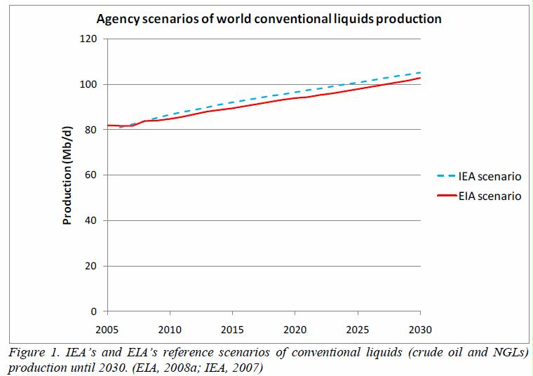
So far both the U.S. Energy Information Administration (EIA) and International Energy Agency (IEA) are on target in their predictions. In 2014 (the last year for which there is data), world production of crude oil and lease condensate was 77.833 million barrels/day (mb/d) and NGL 10.133 mb/d

But the production line may not keep going up until 2030. This paper criticizes the models and methods used by the EIA/IEA to assume growth to 2030.  Much of the paper requires a high mathematical literacy, so I’ve left much of that out – do read the paper in its entirety if you are good at math. ]

Excerpts from:

Jakobsson, K., Söderbergh, B., Höök, M. & Aleklett, K. How reasonable are oil production scenarios from public agencies? Energy Policy, 2009, Vol. 37, Issue 11: 4809-4818, 23 pages 

Abstract. According to the long term scenarios of the  IEA) and the EIA, conventional oil production is expected to grow until at least 2030. EIA has published results from a resource constrained production model which ostensibly supports such a scenario. The model is here described and analyzed in detail. However, it is shown that the model, although sound in principle, has been misapplied due to a confusion of resource categories. A correction of this methodological error reveals that EIA’s scenario requires rather extreme and implausible assumptions regarding future global decline rates. This result puts into question the basis for the conclusion that global “peak oil” would not occur before 2030.

Introduction

For good policymaking, it is important to have good scenarios of the future. A good scenario, we take as evident, is one that builds on reasonable assumptions in the light of past experience. As for global oil production, the most widely cited and authoritative long term scenarios are those published by the International Energy Agency (IEA) of the OECD, and the Energy Information Administration (EIA) of the U.S. Department of Energy. According to the latest available scenarios of conventional crude oil and natural gas liquids supply (as of September 2008), IEA expects production to grow by 1.1% annually, reaching 105 million barrels per day (Mb/d) in 2030; while EIA projects a 1.0% annual increase to 103 Mb/d in 2030. In other words, these two agencies present virtually identical pictures of the future. There will be no peak oil before 2030.

It is relevant, then, to ask how solid the assumptions behind these scenarios really are. EIA’s first long term oil supply scenarios, which must be interpreted as the methodological basis for the optimistic 2030 outlook, were published in 2000 (Wood and Long) and were criticized for being flawed and overly optimistic by Bentley (2002) among others. Four years later, EIA published a new version, virtually identical to the original, stating that “nothing has happened, nor has any new information become available, that would significantly alter the results.” (Wood et al., 2004) The debate on the issue is, in other words, not yet closed. The two main conclusions of this paper are that:

• EIA has taken a generally sound forecasting model and implemented it in a seriously flawed way.
• A correct implementation of the model, using the same assumptions as EIA, indicates that the official scenarios are not reasonable, since oil production can be expected to decline before 2030, possibly in the immediate future.

It should be stressed that the purpose has not been to pin down the exact date of peak oil, but to examine the validity of current forecasts and their underlying assumptions. Transparency has been a high priority, since much of the debate around peak oil appears to stem from either reference to contradictory (and sometimes proprietary) reserve data or from ambiguous use of common terms such as reserves, resources, and depletion.

All data that is referred to in this paper is available in the public domain, and terms are unambiguously defined to the largest extent possible. All references to “oil” implies conventional crude oil, not including natural gas liquids (NGLs), tar sands, extra heavy oil, biofuels or synthetic crude. The volumetric unit of measure is a barrel, which equals 159 liters or 42 U.S. gallons. The abbreviations Gb (billion barrels) and Mb (million barrels) are occasionally used.

Merely presenting a critique of EIA’s forecasting methodology requires only a short paper. The reader who only looks for this specific critique can jump directly to section 6. However, neither EIA, nor any other forecaster, has explained why the applied forecasting method is relevant to begin with. Since we have found the model applied by EIA to be very useful when implemented correctly, especially for field-by-field modeling, we believe that such an explanation is called for. We will therefore first argue for the use of resource constrained modeling in general, describe how this particular model is implemented and point to empirical evidence which justifies its use.

A defense of resource constrained modeling

The forecasting method applied by EIA in Wood et al. (2004), which we in the following will refer to as the Maximum Depletion Rate Model, can be characterized as resource constrained in the sense that the amount of oil in the ground ultimately puts a limit to the rate of production.

The application of resource constrained models is still surrounded by controversy. As the geologist Hubbert put it, the production of a fixed resource must start at zero and also decline to zero, after passing through one or several maxima. (Hubbert, 1956) The peaking phenomenon is thus a trivial consequence of oil’s finite nature.

A meticulous observer could add that no resource is literally exhaustible. (Houthakker, 2002) However, this merely implies that production drops to insignificance without ever becoming identically zero, hardly a distinction of much practical interest.  Adelman has questioned Hubbert’s fundamental assumption by stating that the amount of mineral in the earth is an irrelevant non-binding constraint to production. (1990) This is true in the very limited sense that we will never recover every last drop of oil from the earth. Non-geological circumstances, yet undefined, will limit the actual global recovery factor. However, the recovery factor being undefined is not to say it is unlimited. It is limited to end up between zero and 100 percent of the earth’s abundance (which in itself is perfectly well defined, although not exactly known). Thus, the fact that the amount of recoverable oil is “undefined” and unknown cannot be an argument against the existence of a production peak.

Watkins has, by following a similar way of argument, suggested an agnostic view on whether technology and new knowledge will forever beat the depletion of oil. (Watkins, 2006) But such agnosticism is only defensible in case we refute the original assumption that oil is finite.

Accepting the peaking concept in principle is one thing; agreeing on a good predictive method is another. Hubbert’s approach to the forecasting problem was to estimate an ultimate recovery from the discovery trend, and assume that production would follow a symmetrical bell-shaped curve. The peak would then occur when 50% of the oil was produced. Watkins has argued that asking a Hubbert curve to handle an economic commodity such as oil is like asking a eunuch to sire a family. (2006) Admittedly the Hubbert curve does not explicitly involve economic variables and provides no explanation for the resulting production pattern. There is no particular reason to believe that the peak would occur at a 50% depletion level, or that the production profile would be symmetrical.(Bardi, 2005) The Hubbert curve should therefore be seen as a strictly empirical rule-of-thumb rather than as a rigorous scientific hypothesis. The question is: what is the alternative to an empirical rule-of-thumb?

Constructing a formal model that includes economic variables is notoriously difficult, as Lynch (2002) describes. He even suggests that it is necessary to resort to simple extrapolation as a forecasting method. Simon (1996) takes a similar position when hesitates that the “economist’s approach” consists of extrapolating trends of past costs into the indefinite future. Simon’s conclusion is that since the cost of oil has generally declined during a long period, it must continue to do so indefinitely.

The first counterargument to this way of reasoning concerns the interpretation of empirical data: is there really a contradiction between, on the one hand, long periods of declining cost and, on the other hand, an ultimate production peak followed by increasing cost? As Reynolds (1999) has shown, there is not necessarily any such contradiction, given that technology is improving and that the producers are uncertain about the actual size of the resource.

The second counterargument concerns the general use of extrapolation as a forecasting method. In a certain sense, all science must be extrapolative. The issue, then, is what to extrapolate. Drawing a declining discovery curve into the future would be consistent both with past experience in oil provinces and with the assumption that there is a finite amount of oil to discover (which does not mean that it is valid to forecast future discoveries by extrapolation, due to continuous reserve growth in existing fields). Extrapolating an increasing production curve indefinitely would fail on the second point. Of course, extrapolating an increasing production trend may work most of the time, and in a short term perspective. But predicting an unavoidable trend shift such as peak oil, by first assuming that no trend shifts exist, is clearly an approach bound to failure.

Any useful production model must incorporate the fact that oil is a resource only existing in a finite amount. While it would be desirable to explicitly model the additional influence of economic and other variables, no one has been able to show that it improves the performance of a resource constrained model to an extent that would justify the increased complexity. There is no denying that factors such as oil price matter. The question is: how much do they matter, and can their impact be quantified with any accuracy? If not, then simple resource constrained models are the only tools available for forecasting. Although they may be too simple to accurately predict the exact date of peak oil, they have the potential to distinguish between reasonable and unreasonable scenarios. From a long term policy planning perspective, this should still be valuable information.

Model description

The Maximum Depletion Rate Model (MDRM), as we have chosen to label it, is a resource constrained production model. It does not assume, like the Hubbert curve, that production growth and decline is symmetrical, or that the production peak occurs at the depletion midpoint, but it assumes that there is a limit to the rate at which the remaining resource can be extracted. The MDRM has been used to forecast global oil production for at least 30 years.  However, no forecaster has actually described the foundations of the model, its strengths and caveats, what choices can be made and how they affect the result.

The resource-production ratio (R/P) denotes the relation between the annual production and the resource base at the beginning of the year in question. A central assumption of the MDRM is the existence of a minimum ratio (R/P)min which constrains production in relation to the available resource base. In other words, only a certain fraction of the remaining resource can be produced during one year.

Resource base

Most of the debate around oil production scenarios stems from ambiguous or disputed assumptions concerning the resource base. Applying the MDRM or publishing an R/P figure without clearly stating the underlying resource base is meaningless, since the result is impossible to interpret. Comparisons of studies are irrelevant unless the same type of resource base is used. We will come back to this point when we discuss the way in which EIA uses the model.

An important distinction regarding the resource base is that between fixed and non-fixed resource numbers. A fixed resource base is a “best estimate” of R0 used throughout both computations of historical R/P values and forecasts. Ultimate recoverable resource (URR) is a widely used notation for such a figure, but we will here use the synonym estimated ultimate recovery (EUR) to emphasize that a static resource base is always an estimate. When EUR refers to a region, it should include an estimate of oil yet undiscovered. The weakness of the EUR is that it only can be validated at hindsight; at the point where no forecast is longer needed. The simplest way to handle this inherent uncertainty is to use a range of possible EUR numbers, a range which should narrow as production proceeds. The great advantage of using a fixed resource base is its simplicity.

When a non-fixed resource base is used, the initial resource estimate R0 is continuously updated through resource revisions. A non-fixed resource base is appealing from a theoretical perspective, since it realistically implies that the amount of undiscovered oil is irrelevant for current production. Since resource estimates are dynamic and subject to economic factors, it has been argued that using a fixed resource base is a methodological error (Lynch, 2002). Unfortunately there are significant drawbacks of using a non-fixed resource base at a global level. The main disadvantage is the limited availability of reliable and comparable reserve data.

In practice, the most widely used data is the “proved reserves” compiled annually by the Oil & Gas Journal. However, these numbers have not been evaluated according to consistent criteria. While U.S. reserves are reported conservatively (so-called 1P reserves), most reserves, particularly within OPEC countries, probably are not. Taken together, the public reserve data is a mixed bag of inconsistent reserve figures of little value for forecasting purposes.

It has been suggested that the “proved + probable” (2P) reserves are more suitable for forecasting (Bentley et al., 2007). 2P reflects the amount of oil that can be produced from discovered fields with at least 50% probability. The 2P reserves for discovered fields should, ideally, not grow with time on average. For a more detailed account of reserve definitions, we refer to SPE (2007). Unfortunately 2P reserves are generally not publicly accessible; most of the data can only be obtained from industry databases at considerable cost.

Another disadvantage with a non-fixed resource base is that future resource revisions must be forecasted, perhaps several decades into the future, in order to construct scenarios. The Workshop on Alternative Energy Strategies (WAES, 1977), which used proved reserves as a non-fixed resource base, assumed that the reserves would grow by 10 to 20 Gb/y until the year 2000 and subsequently approach a global EUR of either 1600, 2000, or 3000 Gb. Using a non-fixed resource base is thus not automatically a way to avoid an EUR figure. While it is possible to model a scenario where reserves grow at an undiminished rate, such an approach does not make much sense in a world with a finite amount of oil. If the resource base is not allowed to grow indefinitely, then an ultimate EUR must be assumed at least implicitly.

We recommend the use of a fixed resource base for the sake of simplicity. The theoretical advantage of a non-fixed resource base is in reality diminished due to the lack of good global data and the need to forecast annual reserve additions as well as an implicit EUR.

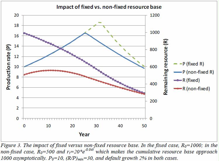
A fixed resource base postpones the peak, but it also results in a steeper decline.

Minimum R/P ratio.  Due to the large number of influencing factors: geological, technological and economic; there is no universal (R/P)min that is applicable to all fields or all regions. After the onset of decline, it is possible to estimate the (R/P)min directly through the observed decline rate. But in the pre-decline phase it is necessary to draw analogies from fields/regions with similar geological and technological conditions.  Estimation of (R/P)min unavoidably involves an element of personal judgment. It is advisable to use a range of possible values rather than one point estimate. All else equal, a lower (R/P)min postpones the peak production and makes the subsequent decline steeper.

Default production curve.  Production is not geologically constrained as long as R/P is higher than the assumed (R/P)min. Therefore, it can actually be quite arbitrarily defined. The two simplest options are either to keep it at a constant plateau level (typical of many individual fields, where the plateau is determined by the technical capacity), or to let it grow at a constant rate (suitable for regions). All else equal, a higher default production rate propones the peak since the resource base is more rapidly depleted.

Calculating R/P for a region.  It is impossible to give an analytical formula for the temporal distribution of fields, since the timing of production from a particular field is determined by the year of discovery, available extraction technology, administrative barriers, macroeconomic circumstances, and other factors. The estimation of (R/P)reg, min must therefore rely on empirical experience of how regions generally develop.

Empirical support for the MDRM

The MDRM (using a fixed resource base) fits well with observed production behavior of individual wells and fields. Arps (1944) described how production unconstrained by capacity limits can be empirically fitted to a hyperbolic decline function

In other words, assuming that there exists an (R/P)min is equivalent to assuming exponential decline. The simplicity of the exponential function has made it a popular forecasting tool within the field of reservoir engineering called decline curve analysis. Under certain ideal reservoir conditions, the exponential behavior can be derived from physical reservoir variables (Fetkovich, 1980). When reservoir conditions are not ideal, the tail end production tends to resemble a hyperbolic or harmonic decline.

Statfjord, Ekofisk, Oseberg and Gullfaks are hitherto the four largest Norwegian fields in terms of original recoverable resources. Since Statfjord, Oseberg and Gullfaks are long past their respective peaks and are estimated to have a depletion level higher than 90%, their EURs are reasonably certain. Ekofisk is estimated to be more than 70% depleted, but the EUR has been revised upwards considerably in the past. All four fields are produced with water and/or gas injection, though at Ekofisk only on a large scale since 1987. Figure 5 shows the production curves together with the fitted (R/P)min. An (R/P)min of 6-7 has been attainable in three of the four cases, and the model fits well with the observed decline. In the case of Ekofisk, subsidence of the seafloor and compaction of the reservoir has led to production difficulties, but also to a substantially increased recovery factor (Nagel, 2001). Such exceptional conditions cannot be captured by the MDRM.

Macro level.  We cannot assume a priori that a model which fits well to individual fields will be useful also at the regional level. Applying a model to aggregated data always leads to loss of information. Whenever possible, we would recommend a field-by-field approach to avoid aggregation. However, that is not a feasible strategy for a global scenario. Fortunately, evidence suggests that the MDRM is reasonably consistent with observed production profiles even for larger regions, which justifies its use also as a global model.

Brandt (2007) used production data from 139 oil producing regions of various sizes, from U.S. state level to continents, in order to test the goodness-of-fit of three simple growth/decline models: Hubbert, linear, and exponential. Brandt also allowed for asymmetrical growth/decline patterns. Several of the results are relevant in this context: In 74 of the 139 regions (53%), both a growth and decline rate could be estimated. Asymmetrical models generally had a better fit than symmetrical ones, even when adjusting for the increased complexity. The Hubbert model (symmetrical or asymmetrical) had the best fit in 19 of the 74 cases (26%), the linear model in 16 cases (22%), and the exponential model in 32 cases (43%). In 7 cases there was no clear best fitting model. There is no evidence that the Hubbert model would fit better to larger regions than smaller ones. Regions generally have a slower decline rate than growth rate. The mean decline rate in the 74 regions was 4.1%, a number inflated by a few extreme cases, since three quarters of the regions showed a rate less than 3.8%. The median rate was 2.6%, while the rate weighted for cumulative production was merely 1.9% which indicates that larger regions tend to decline more slowly than smaller ones.

The exponential growth/decline model, which was the single best-fitting of the models tested, is consistent with the MDRM. Brandt’s results can therefore be taken as an indication that the MDRM is at least as good as other simple resource constrained models at a regional level. The observed decline rates suggest that larger region size is related to slower decline. This is consistent with the discussion about regional (R/P)min in section 3.3. The observed decline rates should be interpreted with some caution, since it is not certain that they will remain unchanged in the future.

Sensitivity and uncertainty

Since R/P is a function of both the production rate and the remaining resource base, uncertainty in any of these two parameters necessarily reduces the reliability of the estimated R/P. In practice, the resource base is the major source of uncertainty. A complicating circumstance is that R/P is disproportionately sensitive to uncertainty in the resource base. Figure 6 illustrates how revisions in a fixed resource base affect the estimated R/P at different depletion levels. The problem does not occur when a non-fixed resource base is used, since current resource revisions do not affect past years’ R/P.

Assume, for example, that the depletion level (based on the original estimate of R0) at the end of year t-1 is 50%, while the estimated R/P at year t is 20. If the estimated R0 is then adjusted 10% upwards, the R/P is altered by a factor of 1.2. The new R/P for year t thus becomes 1.2*20=24.

At high depletion levels the R/P is very sensitive to even small uncertainties in the resource base. For this reason, one should not put too much weight on the R/P at high levels of depletion. The absolute level of production is usually low at this stage in any case, so a precise estimate of R/P is not necessary. What matters most is the R/P at peak/end-of-plateau, which typically occurs when the depletion level is 30-60% (see figure 7).

EIA’s long term world oil supply scenarios

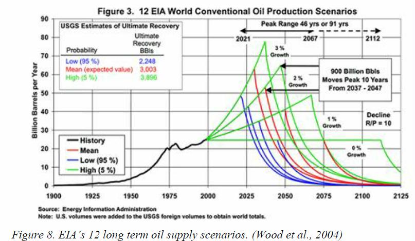
The conclusion of the 2004 EIA report is that peak oil is not imminent, however very likely to occur within a century. Twelve scenarios are generated, using combinations of three different resource estimates and four alternative growth rates until peak (0-3%). The resource estimates are the low (2248 Gb), medium (3003 Gb) and high (3896 Gb) scenarios from the World Petroleum Assessment of the U.S. Geological Survey (USGS, 2000), which estimated the amount of conventional oil and NGL that would be made available through new discoveries and reserve appreciation until 2025 in the world exclusive of the U.S. To these figures, EIA has added their own resource estimates for the U.S. Subtracting USGS’s estimates from the total indicates that the range of the U.S. resource base, according to EIA, is 324-360 Gb, with 344 Gb as a mean estimate. Regarding the decline behavior post-peak, only one scenario is considered and motivated in the following way:

EIA selected an R/P ratio of 10 as being representative of the post-peak production experience. The United States, a large, prolific, and very mature producing region, has an R/P ratio of about 10 and was used as the model for the world in a mature state” (Wood et al., 2004).

The result is summarized in figure 8. The peak dates are spread out over the time span 2021-2112, but 2037 is pointed out as a reference case.

There are indeed significant uncertainties regarding the resource base and future demand growth. The result is thus a combined scenario and sensitivity analysis. It is however striking that no alternative decline behaviors have been considered. There can only be two justifiable arguments for their absence: (1) there is virtually no uncertainty in the assumed decline behavior; (2) although there are uncertainties, they have no significant impact on the timing of the peak. Both these potential arguments are unfounded.

The resource base for the forecast is estimates of global EUR. EIA does not explicitly state that they use a fixed resource base, but it appears reasonable since they do not assume any resource growth rate. But when the EIA points to the U.S. as an analogous case, they refer to the R/P based on proved reserves, a resource base which is non-fixed and has grown considerably in the past. It is true that the U.S. R/P based on proved reserves have fluctuated around 10 for several decades, but that is irrelevant in this context. A relevant analogy would be the U.S. (R/P)min computed from the same resource base that EIA assumes in their forecast (324-360 Gb EUR), which would yield an (R/P)min of around 70 rather than 10 (see figure 9). USA:

The resource base

Another factor not related to EIA’s methodology, but still crucial for the result, is the resource estimates generated by the U.S. Geological Survey. The mean estimate implies that the world’s total reserves (outside the U.S.) will grow by 1261 Gb during the period 1996-2025. 649 Gb will be new discoveries of conventional oil, 612 Gb reserve growth in known fields. The majority of other recent estimates of global EUR fall within the span set by the high and low estimates of USGS (NPC, 2007). However, an evaluation of the petroleum assessment (Klett et al., 2007) indicates that between 1996 and 2003 (27% of the assessment period) only 69 Gb (11% of 649 Gb) was discovered. It appears motivated to conclude that USGS’s mean and high resource estimates are unconfirmed and may be over-optimistic. The current discovery rate indicates that the low estimate (334 Gb until 2025) should be considered more likely. The reserve growth, on the other hand, was of the expected magnitude (171 Gb, or 28%). Almost half of this reserve growth has occurred in Middle East and North Africa. Since USGS did not publish reserve growth estimates for individual regions, it is impossible to determine whether the result actually validates the estimation method or is merely a coincidence.

Alternative world oil scenarios

Our world oil supply scenarios are applications of the MDRM, like those of EIA, but with some important modifications. While EIA used an invalid (R/P)min and did not examine how different values affected the result, it is here shown that the assumed (R/P)min has a dramatic impact on the timing of the peak. The scenarios display values of (R/P)min ranging from 70 to 30. The upper limit is what has been observed historically in the U.S.; the lower limit implies that the world should have a 3.3% decline rate, which appears rather extreme compared to the regional decline rates presented by Brandt (2007) and the fact that larger regions tend to decline more slowly than smaller ones. A reasonable guess is that the actual value will be within the range 70-50.

For each (R/P)min scenario there are three alternative EUR estimates. We use the same low (2248 Gb), mean (3003 Gb) and high (3896 Gb) estimates as EIA for the sake of comparability, although the mean and high estimates seem rather optimistic in the light of current discovery rates.

Since the main purpose of the study is to examine the realism of official production forecasts, the demand growth is always assumed to be 1% annually, which is the demand growth rate that EIA and IEA project until 2030. The official forecasts include both crude oil and NGLs, while our scenarios only concern crude oil in order to be comparable with Wood et al. (2004). We have made the simplifying assumption that crude oil and NGLs will grow proportionately.

The world production in 2007 was 26.7 Gb according to EIA statistics. We estimate the cumulative production at the end of 2007 to be 1012 Gb based on the USGS Petroleum Assessment and more recent production figures from EIA.

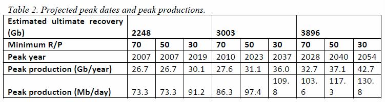
The result is shown in figure 10 and summarized in table 2. The projected peak dates range from 2007 to 2054.

Assuming EUR = 2248 Gb and (R/P)min = 70, production collapses immediately which indicates that at least one of the parameters is incorrect.

The significant result, however, is that sustained production growth to 2030 requires either that the (R/P)min is 30 together with an EUR of at least 3003 Gb, or else that the EUR must be 3896 Gb. It thus appears likely that crude oil production will start to decline before 2030. An imminent peak in production cannot be ruled out.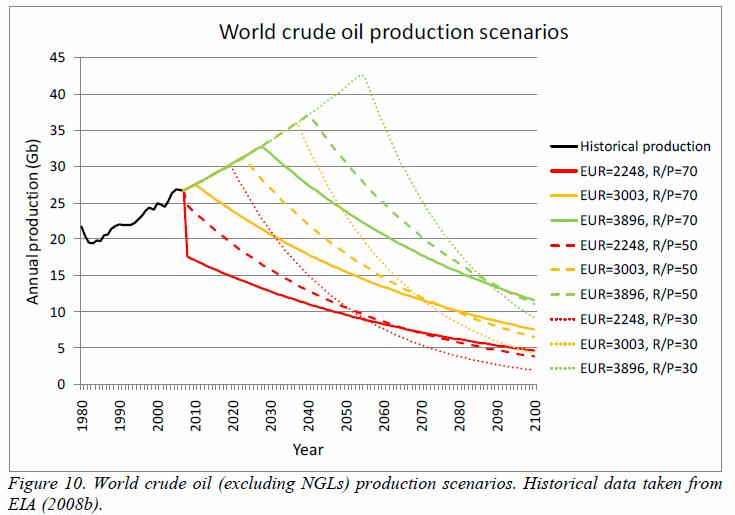

The present study has indicated that:

1. Resource constrained models are presently the only feasible tools for long term oil production scenarios.
2. The best way to account for uncertainty is to use a range of values for all relevant parameters.
3. The Maximum Depletion Rate Model (MDRM) is consistent with empirical experience at the field level, and is at least as good as other resource constrained models at a regional level. It is therefore reasonable to use it for global scenarios.
4. Using a fixed resource base (EUR estimates) yields an exponential decline behavior and is preferable over a non-fixed resource base from a practical point of view.
5. EIA has constructed unreasonable world scenarios by making an invalid analogy between R/P based on “proved reserves” and R/P based on EUR.
6. A correct implementation of the model shows that crude oil production may start to decline well before 2030. An imminent peak cannot be ruled out.
7. The result puts into question the reasonability of EIA’s and IEA’s official production forecasts, which assume that oil production will grow by 1% annually at least until 2030.

In the peak oil debate, analysts who downplay the possibility of an early peak are usually labeled “optimists”. This title we would like to claim for ourselves. In our view, optimism means to always have a constructive attitude after a sober look at the facts at hand, not merely hope for the best scenario to come about. An early production peak followed by a gentle decline should provide good opportunities for an orderly transition from today’s oil dependent economy to a more sustainable one. It should definitely not be interpreted as a doomsday scenario, but rather as a cause for cautious optimism. EIA’s high-peak-steep-decline scenarios, on the other hand, would make an orderly transition extremely difficult and likely have catastrophic consequences for the economy.

References

• Adelman, M.A., 1990. Mineral depletion, with special reference to petroleum, Review of Economics & Statistics, pp. 1-10.
• Arps, J.J., 1944. Analysis of decline curves (Technical Publication no. 1758). American Institute of Mining and Metallurgical Engineers.
• Bardi, U., 2005. The mineral economy: a model for the shape of oil production curves. Energy Policy 33, 53-61.
• Bentley, R.W., 2002. Global oil & gas depletion: an overview. Energy Policy 30, 189-205.
• Bentley, R.W., Mannan, S.A., Wheeler, S.J., 2007. Assessing the date of the global oil peak: The need to use 2P reserves. Energy Policy 35, 6364-6382.
• Brandt, A.R., 2007. Testing Hubbert. Energy Policy 35, 3074-3088.
• Energy Information Administration (EIA), 2008a. International Energy Outlook 2008. Energy Information Administration, Washington, DC.
• Energy Information Administration (EIA), 2008b. Petroleum Navigator. Energy Information Administration.
• Fetkovich, M.J., 1980. Decline curve analysis using type curves. Journal of Petroleum Technology June 1980, 1065-1077.
• Flower, A.R., 1978. World oil production. Scientific American 238, 42-49.
• Houthakker, H.S., 2002. Are Minerals Exhaustible? Quarterly Review of Economics and Finance 42, 417-421.
• Hubbert, M.K., 1956. Nuclear energy and the fossil fuels. Shell Development Company, Exploration and Production Research Division, Houston.
• International Energy Agency (IEA), 2007. World Energy Outlook 2007. OECD/International Energy Agency, Paris.
• Klett, T.R., Gautier, D.L., Ahlbrandt, T.S., 2007. An Evaluation of the USGS World Petroleum Assessment 2000 – Supporting Data. U.S. Geological Survey Open-File Report 2007-1021.
• Lynch, M.C., 2002. Forecasting oil supply: theory and practice. The Quarterly Review of Economics and Finance 42, 373-389.
• Nagel, N.B., 2001. Compaction and subsidence issues within the petroleum industry: From Wilmington to Ekofisk and beyond. Physics and Chemistry of the Earth, Part A: Solid Earth and Geodesy 26, 3-14.
• National Petroleum Council (NPC), 2007. Facing the Hard Truths about Energy. National Petroleum Council, Washington, D.C.
• Norwegian Petroleum Directorate (NPD), 2008. Fact Pages. Norwegian Petroleum Directorate.
• Reynolds, D.B., 1999. The mineral economy: how prices and costs can falsely signal decreasing scarcity. Ecological Economics 31, 155-166.
• Simon, J., 1996. The Ultimate Resource 2, 2 ed. Princeton University Press, Princeton.
• Society of Petroleum Engineers (SPE), 2007. Petroleum Resources Management System. Society of Petroleum Engineers.
• United States Geological Survey (USGS), 2000. World Petroleum Assessment 2000. USGS.
• Watkins, G.C., 2006. Oil scarcity: What have the past three decades revealed? Energy Policy 34, 508-514.
• Wood, J.H., Long, G.R., 2000. Long Term World Oil Supply (A Resource Based / Production Path Analysis). Energy Information Administration.
• Wood, J.H., Long, G.R., Morehouse, D.F., 2004. Long-Term World Oil Supply Scenarios: The Future is Neither as Bleak or Rosy as Some Assert. Energy Information Administration.
• Workshop on Alternative Energy Strategies (WAES), 1977. Energy Supply to the Year 2000: Global and National Studies. The MIT Press, Cambridge, Mass.