Preface. This is a summary of the National Research Council 2013 study of abrupt changes of climate change.

Related:

2019-12-6. Research reveals past rapid Antarctic ice loss due to ocean warming.  “…the sensitive West Antarctic Ice Sheet collapsed during a warming period just over a million years ago when atmospheric carbon dioxide levels were lower than today.”

2015-8-5. The Point of No Return: Climate Change Nightmares Are Already Here.  The worst predicted impacts of climate change are starting to happen — and much faster than climate scientists expected. Rolling Stone.

Alice Friedemann   www.energyskeptic.com  author of “When Trucks Stop Running: Energy and the Future of Transportation”, 2015, Springer, Barriers to Making Algal Biofuels, and “Crunch! Whole Grain Artisan Chips and Crackers”. Podcasts: Collapse Chronicles, Derrick Jensen, Practical Prepping, KunstlerCast 253, KunstlerCast278, Peak Prosperity , XX2 report

***

NRC. 2013. Abrupt Impacts of Climate Change: Anticipating surprises. National Research Council, National Academies of Sciences press.

“Abrupt climate change is generally defined as occurring when some part of the climate system passes a threshold or tipping point resulting in a rapid change that produces a new state lasting decades or longer (Alley et al., 2003). In this case “rapid” refers to timelines of a few years to decades.

“Abrupt climate change can occur on a regional, continental, hemispheric, or even global basis. Even a gradual forcing of a system with naturally occurring and chaotic variability can cause some part of the system to cross a threshold, triggering an abrupt change. Therefore, it is likely that gradual or monotonic forcings increase the probability of an abrupt change occurring.

Climate is changing, forced out of the range of the last million years by levels of carbon dioxide and other greenhouse gases not seen in Earth’s atmosphere for a very long time.

It is clear that the planet will be warmer, sea level will rise, and patterns of rainfall will change. But the future is also partly uncertain—there is considerable uncertainty about how we will arrive at that different climate. Will the changes be gradual, allowing natural systems and societal infrastructure to adjust in a timely fashion? Or will some of the changes be more abrupt, crossing some threshold or “tipping point” to change so fast that the time between when a problem is recognized and when action is required shrinks to the point where orderly adaptation is not possible?

A study of Earth’s climate history suggests the inevitability of “tipping points”— thresholds beyond which major and rapid changes occur when crossed—that lead to abrupt changes in the climate system.

The history of climate on the planet—as read in archives such as tree rings, ocean sediments, and ice cores—is punctuated with large changes that occurred rapidly, over the course of decades to as little as a few years.

There are many potential tipping points in nature, as described in this report, and many more that we humans create in our own systems. The current rate of carbon emissions is changing the climate system at an accelerating pace, making the chances of crossing tipping points all the more likely.

Scientific research has already helped us reduce this uncertainty in two important cases; potential abrupt changes in ocean deep water formation and the release of carbon from frozen soils and ices in the polar regions were once of serious near-term concern are now understood to be less imminent, although still worrisome as slow changes over longer time horizons. In contrast, the potential for abrupt changes in ecosystems, weather and climate extremes, and groundwater supplies critical for agriculture now seem more likely, severe, and imminent.

In addition to a changing climate, multiple other stressors are pushing natural and human systems toward their limits, and thus become more sensitive to small perturbations that can trigger large responses. Groundwater aquifers, for example, are being depleted in many parts of the world, including the southeast of the United States. Groundwater is critical for farmers to ride out droughts, and if that safety net reaches an abrupt end, the impact of droughts on the food supply will be even larger.

Levels of carbon dioxide and other greenhouse gases in Earth’s atmosphere are exceeding levels recorded in the past millions of years, and thus climate is being forced beyond the range of the recent geological era.

The paleoclimate record—information on past climate gathered from sources such as fossils, sediment cores, and ice cores—contains ample evidence of abrupt changes in Earth’s ancient past, including sudden changes in ocean and air circulation, or abrupt extreme extinction events. One such abrupt change was at the end of the Younger Dryas, a period of cold climatic conditions and drought in the north that occurred about 12,000 years ago. Following a millennium-long cold period, the Younger Dryas abruptly terminated in a few decades or less and is associated with the extinction of 72 percent of the large-bodied mammals in North America. Some abrupt climate changes are already underway, including the rapid decline of Arctic sea ice over the past decade due to warmer polar temperatures.

Scientific research has advanced sufficiently that it is possible to assess the likelihood, for example the probability of a rapid shutdown of the Atlantic Meridional Overturning Circulation (AMOC) within this century is now understood to be low.

Human infrastructure is built with certain expectations of useful life expectancy, but even gradual climate changes may trigger abrupt thresholds in their utility, such as rising sea levels surpassing sea walls or thawing permafrost destabilizing pipelines, buildings, and roads.

The primary timescale of concern is years to decades. A key characteristic of these changes is that they can come faster than expected, planned, or budgeted for, forcing more reactive, rather than proactive, modes of behavior.

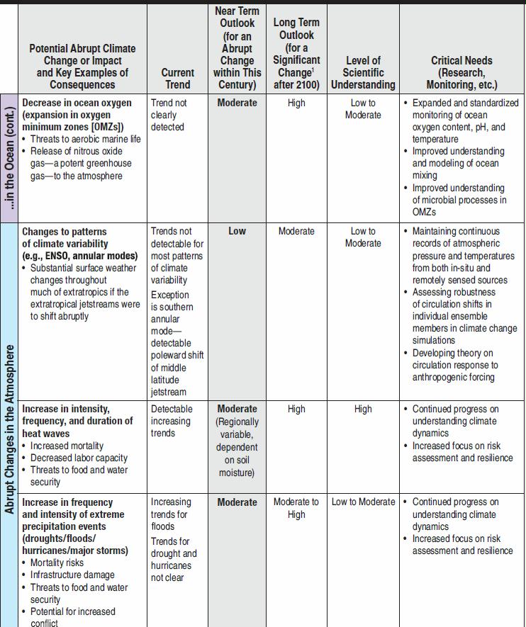
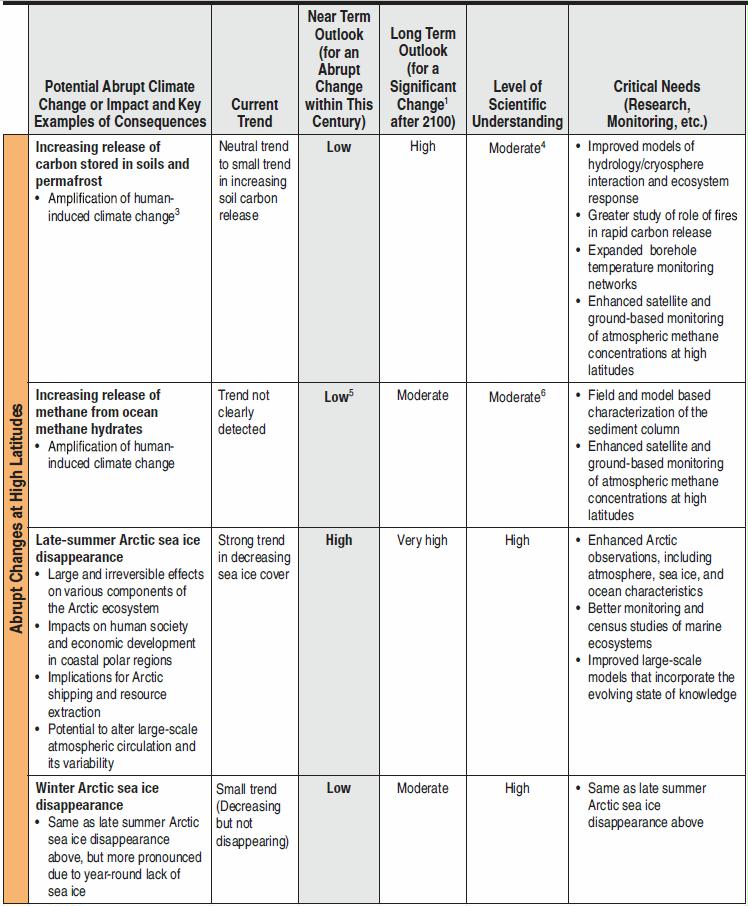
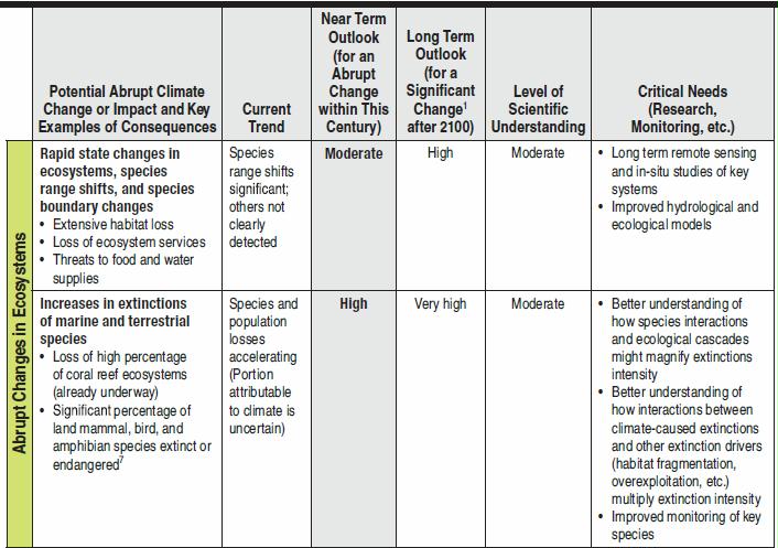
Table S.1 summarizes the state of knowledge about potential abrupt changes. This table includes potential abrupt changes to the ocean, atmosphere, ecosystems, and highlatitude regions that are judged to meet the above criteria. For each abrupt change, the Committee examined the available evidence of potential impact and likelihood. Some abrupt changes are likely to occur within this century—making these changes of most concern for near-term societal decision making and a priority for research.

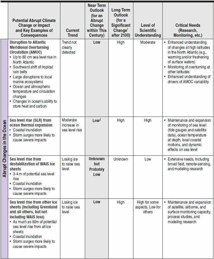
1 Change could be either abrupt or non-abrupt.

2 Committee assesses the near-term outlook that sea level will rise abruptly before the end of this century as Low; this is not in contradiction to the assessment that sea level will continue to rise steadily with estimates of between 0.26 and

0.82­m by the end of this century (IPCC, 2013).

3 Methane is a powerful but short-lived greenhouse gas

4 Limited by ability to predict methane production from thawing organic carbon

5 No mechanism proposed would lead to abrupt release of substantial amounts of methane from ocean methane hydrates this century.

6 Limited by undertainty in hydrate abundance in near-surface sediments, and fate of CH4 once released

7 Species distribution models (Thuiller et al., 2006) indicate between 10–40% of mammals now found in African protected areas will be extinct or critically endangered by 2080 as a result of modeled climate change. Analyses by Foden et al.(2013) and Ricke et al. (2013) suggest 41% of bird species, 66% of amphibian species, and between 61% and 100% of corals that are not now considered threatened with extinction will become threatened due to climate change sometime between now and 2100.

Disappearance of Late-Summer Arctic Sea Ice

Recent dramatic changes in the extent and thickness of the ice that covers the Arctic sea have been well documented. Satellite data for late summer (September) sea ice extent show natural variability around a clearly declining long-term trend (Figure S.1). This rapid reduction in Arctic sea ice already qualifies as an abrupt change with substantial decreases in ice extent occurring within the past several decades. Projections from climate models suggest that ice loss will continue in the future, with the full disappearance of late-summer Arctic sea ice possible in the coming decades. The impacts of rapid decreases in Arctic sea ice are likely to be considerable. More open water conditions during summer would have potentially large and irreversible effects on various components of the Arctic ecosystem, including disruptions in the marine food web, shifts in the habitats of some marine mammals, and erosion of vulnerable coastlines. Because the Arctic region interacts with the large-scale circulation systems of the ocean and atmosphere, changes in the extent of sea ice could cause shifts in climate and weather around the northern hemisphere. The Arctic is also a region of increasing economic importance for a diverse range of stakeholders, and reductions in Arctic sea ice will bring new legal and political challenges as navigation routes for commercial shipping open and marine access to the region increases for offshore oil and gas development, tourism, fishing and other activities.

Increases in Extinction Threat for Marine and Terrestrial Species

The rate of climate change now underway is probably as fast as any warming event in the past 65 million years, and it is projected that its pace over the next 30 to 80 years will continue to be faster and more intense. These rapidly changing conditions make survival difficult for many species. Biologically important climatic attributes—such as number of frost-free days, length and timing of growing seasons, and the frequency and intensity of extreme events (such as number of extremely hot days or severe storms)—are changing so rapidly that some species can neither move nor adapt fast enough

The distinct risks of climate change exacerbate other widely recognized and severe extinction pressures, especially habitat destruction, competition from invasive species, and unsustainable exploitation of species for economic gain, which have already elevated extinction rates to many times above background rates. If unchecked, habitat destruction, fragmentation, and over-exploitation, even without climate change, could result in a mass extinction within the next few centuries equivalent in magnitude to the one that wiped out the dinosaurs. With the ongoing pressures of climate change, comparable levels of extinction conceivably could occur before the year 2100; indeed, some models show a crash of coral reefs from climate change alone as early as 2060 under certain scenarios. Loss of a species is permanent and irreversible, and has both economic impacts and ethical implications. The economic impacts derive from loss of ecosystem services, revenue, and jobs, for example in the fishing, forestry, and ecotourism industries. Ethical implications include the permanent loss of irreplaceable species and ecosystems as the current generation’s legacy to the next generation.

Abrupt Changes of Unknown Probability Destabilization of the West Antarctic Ice Sheet

The volume of ice sheets is controlled by the net balance between mass gained (from snowfall that turns to ice) and mass lost (from iceberg calving and the runoff of meltwater from the ice sheet). Scientists know with high confidence from paleo-climate records that during the planet’s cooling phase, water from the ocean is traded for ice on land, lowering sea level by tens of meters or more, and during warming phases, land ice is traded for ocean water, raising sea level, again by tens of meters and more. The rates of ice and water loss from ice stored on land directly affect the speed of sea level rise, which in turn directly affects coastal communities. Of greatest concern among the stocks of land ice are those glaciers whose bases are well below sea level, which includes most of West Antarctica, as well as smaller parts of East Antarctica and Greenland. These glaciers are sensitive to warming oceans, which help to thermally erode their base, as well as rising sea level, which helps to float the ice, further destabilizing them. Accelerated sea level rise from the destabilization of these glaciers, with sea level rise rates several times faster than those observed today, is a scenario that has the potential for very serious consequences for coastal populations, but the probability is currently not well known,

Research to understand ice sheet dynamics is particularly focused on the boundary between the floating ice and the grounded ice, usually called the grounding line (see Figure S.3). The exposed surfaces of ice sheets are generally warmest on ice shelves, because these sections of ice are at the lowest elevation, furthest from the cold central region of the ice mass and closest to the relatively warmer ocean water. Locations where meltwater forms on the ice shelf surface can wedge open crevasses and cause ice-shelf disintegration—in some cases, very rapidly.

Because air carries much less heat than an equivalent volume of water, physical understanding indicates that the most rapid melting of ice leading to abrupt sea-level rise is restricted to ice sheets flowing rapidly into deeper water capable of melting ice rapidly and carrying away large volumes of icebergs. In Greenland, such deep water contact with ice is restricted to narrow bedrock troughs where friction between ice and fjord walls limits discharge. Thus, the Greenland ice sheet is not expected to destabilize rapidly within this century. However, a large part of the West Antarctic Ice Sheet (WAIS), representing 3–4 m of potential sea-level rise, is capable of flowing rapidly into deep ocean basins. Because the full suite of physical processes occurring where ice meets ocean is not included in comprehensive ice-sheet models, it remains possible that future rates of sea-level rise from the WAIS are underestimated, perhaps substantially.

Abrupt Changes Unlikely to Occur This Century

These include disruption to the Atlantic Meridional Overturning Circulation (AMOC) and potential abrupt changes of high-latitude methane sources (permafrost soil carbon and ocean methane hydrates). Although the Committee judges the likelihood of an abrupt change within this century to be low for these processes, should they occur even next century or beyond, there would likely be severe impacts. Furthermore, gradual changes associated with these processes can still lead to consequential changes.

However, it is important keep a close watch on this system, to make observations of the North Atlantic to monitor how the AMOC responds to a changing climate, for reasons including the likelihood that slow changes will have real impacts, and to update the understanding of the slight possibility of a major event.

Potential Abrupt Changes due to High-Latitude Methane

Large amounts of carbon are stored at high latitudes in potentially labile reservoirs such as permafrost soils and methane-containing ices called methane hydrate or clathrate, especially offshore in ocean marginal sediments. Owing to their sheer size, these carbon stocks have the potential to massively affect Earth’s climate should they somehow be released to the atmosphere. An abrupt release of methane is particularly worrisome because methane is many times more potent than carbon dioxide as a greenhouse gas over short time scales. Furthermore, methane is oxidized to carbon dioxide in the atmosphere, representing another carbon dioxide pathway from the biosphere to the atmosphere.

According to current scientific understanding, Arctic carbon stores are poised to play a significant amplifying role in the century-scale buildup of carbon dioxide and methane in the atmosphere, but are unlikely to do so abruptly, i.e., on a timescale of one or a few decades.

Although comforting, this conclusion is based on immature science and sparse monitoring capabilities. Basic research is required to assess the long-term stability of currently frozen Arctic and sub-Arctic soil stocks, and of the possibility of increasing the release of methane gas bubbles from currently frozen marine and terrestrial sediments, as temperatures rise.

The Committee examined a number of other possible changes. These included sea level rise due to thermal expansion or ice sheet melting (except WAIS—see above), decrease in ocean oxygen (expansion in oxygen minimum zones (OMZs)), changes to patterns of climate variability, changes in heat waves and extreme precipitation events (droughts/floods/ hurricanes/major storms), disappearance of winter Arctic sea ice (distinct from late summer Arctic sea ice—see above), and rapid state changes in ecosystems, species range shifts, and species boundary changes.

Early studies of ice cores showed that very large changes in climate could happen in a matter of a few decades or even years, for example, local to regional temperature changes of a dozen degrees or more, doubling or halving of precipitation rates, and dust concentrations changing by orders of magnitude

What has become clearer recently is that the issue of abrupt change cannot be confined to a geophysical discussion of the climate system alone. The key concerns are not limited to large and abrupt shifts in temperature or rainfall, for example, but also extend to other systems that can exhibit abrupt or threshold-like behavior even in response to a gradually changing climate. The fundamental concerns with abrupt change include those of speed—faster changes leave less time for adaptation, either economically or ecologically—and of magnitude—larger changes require more adaptation and generally have greater impact.

This report offers an updated look at the issue of abrupt climate change and its potential impacts, and takes the added step of considering not only abrupt changes to the climate system itself, but also abrupt impacts and tipping points that can be triggered by gradual changes in climate. This examination of the impacts of abrupt change brings the discussion into the human realm, raising questions such as: Are there potential thresholds in society’s ability to grow sufficient food? Or to obtain sufficient clean water? Are there thresholds in the risk to coastal infrastructure as sea levels rise?

Bark beetles are a natural part of forested ecosystems, and infestations are a regular force of natural change. In the last two decades, though, the bark beetle infestations that have occurred across large areas of North America have been the largest and most severe in recorded history, killing millions of trees across millions of hectares of forest from Alaska to southern California (Bentz, 2008); see Figure B. Bark beetle outbreak dynamics are complex, and a variety of circumstances must coincide and thresholds must be surpassed for an outbreak to occur on a large scale. Climate change is thought to have played a significant role in these recent outbreaks by maintaining temperatures above a threshold that would normally lead to cold-induced mortality.

When there are consecutive warm years, this can speed up reproductive cycles and increase the likelihood of outbreaks (Bentz et al., 2010). Similar to many of the issues described in this report, climate change is only one contributing factor to these types of abrupt climate impacts, with other human actions such as forest history and management also playing a role.

They noted that events that did not meet the common criterion of a semi-permanent change in state could still force other systems into a permanent change, and thus qualify as an abrupt change. For example, a mega-drought may be followed by the return of normal precipitation rates, such that no baseline change occurred, but if that drought caused the collapse of a civilization, a permanent, abrupt change occurred in the system impacted by climate.

The 2002 NRC study introduced the important issue of gradual climate change causing abrupt responses in human or natural systems, noting “Abrupt impacts therefore have the potential to occur when gradual climatic changes push societies or ecosystems across thresholds and lead to profound and potentially irreversible impacts.” The 2002 report also noted that “…the more rapid the forcing, the more likely it is that the resulting change will be abrupt on the time scale of human economies or global ecosystems” and “The major impacts of abrupt climate change are most likely to occur when economic or ecological systems cross important thresholds

Changes occurring over a few decades, i.e., a generation or two, begin to capture the interest of most people because it is a time frame that is considered in many personal decisions and relates to personal memories. Also, at this time scale, changes and impacts can occur faster than the expected, stable lifetime of systems about which society cares. For example, the sizing of a new air conditioning system may not take into consideration the potential that climate change could make the system inadequate and unusable before the end of its useful lifetime (often 30 years or more). The same concept applies to other infrastructure, such as airport runways, subway systems, and rail lines. Thus, even if a change is occurring over several decades, and therefore might not at first glance seem “abrupt,” if that change affects systems that are expected to function for an even longer period of time, the impact can indeed be abrupt when a threshold is crossed. “Abrupt” then, is relative to our “expectations,” which for the most part come from a simple linear extrapolation of recent history, and “expectations” invoke notions of risk and uncertainty. In such cases, it is the cost associated with unfulfilled expectations that motivates discussion of abrupt change. Finally, changes occurring over one to a few years are abrupt, and for most people, would also be alarming if sufficiently large and impactful.

The rate of greenhouse gas addition to the atmosphere continues to increase, with many policies in place to accelerate rising greenhouse gases (IMF, 2013). It is sobering to consider that about one-fifth of all fossil fuels ever burned were burned since the 2002 report was released. The sum of global emissions from 1751 through 2009 inclusive is 355,676 million metric tons of carbon; sum of global emissions from 2002 through 2009 inclusive is 64,788 million metric tons of carbon (Boden et al., 2011). Total carbon emissions for 2002-2009 compared to the total 1751-2009 is thus greater than 18%.

Abrupt Changes of Primary Concern

Either because they are currently believed to be the most likely and the most impactful, because they are predicted to potentially cause severe impacts but with uncertain likelihood, or because they are considered to be unlikely to occur but have been widely discussed in the literature or media.

It is very unlikely that the AMOC will undergo an abrupt transition or collapse in the 21st century. Delworth et al. (2008) pointed out that for an abrupt transition of the AMOC to occur, the sensitivity of the AMOC to forcing would have to be far greater than that seen in current models. Alternatively, significant ablation of the Greenland ice sheet greatly exceeding even the most aggressive of current projections would be required. As noted in the ice sheet section later in this chapter, Greenland ice has about 7.3m equivalent of sea level rise, which, if melted over 1000 years, yields an annual rise rate of 7 mm/yr, about 2 times faster just from Greenland than today’s rate from all sources, and more than 10 times faster than the rate from Greenland over 2000–2011 (Shepherd et al., 2012). Although neither possibility can be excluded entirely, it is unlikely that the AMOC will collapse before the end of the 21st century because of global warming.

Rising sea level increases the likelihood that a storm surge will overtop a levee or damage other coastal infrastructure, such as coastal roads, sewage treatment plants, or gas lines—all with potentially large, expensive, and immediate consequences

A separate but key question is whether sea-level rise itself can be large, rapid and widespread. In this regard, rate of change is assessed relative to the rate of societal adaptation. Available scientific understanding does not answer this question fully, but observations and modeling studies do show that a much faster sea-level rise than that observed recently (~3 mm/yr over recent decades) is possible (Cronin, 2012). Rates peaked more than 10 times faster in Meltwater Pulse 1A during the warming from the most recent ice age, a time with more ice on the planet to contribute to the sealevel rise, but slower forcing than the human-caused rise in CO2 (Figure 2.5 and 2.6). One could term a rise “rapid” if the response or adaptation time is significantly longer than the rise time. For example, a rise rate of 15 mm/yr (within the range of projec

Projections of sea-level rise remain notably uncertain even if the increase in greenhouse gases is specified accurately, but many recently published estimates include within their range of possibilities a rise of 1m by the end of this century (reviewed by Moore et al., 2013). For lowlying metropolitan areas, such as Miami and San Francisco, such a rise could lead to significant flooding

Thirty nine percent of the population lives in coastal shoreline counties. This population grew by 39 percent between 1970 and 2010, and is projected to grow by 8.3 percent by 2020. The population density of coastal counties is 446 people per sq mile, which is over 4 times that of inland counties. Just under half of the annual GDP of the United States is generated in coastal shoreline counties, an annual contribution that was $6.6 trillion in 2011. If counted as their own country, these counties would rank as the world’s third largest economy, after the United States and China. Some portions of these counties are well above sea level and not vulnerable to flooding (e.g., Cadillac Mountain, Maine, in Acadia National Park, at 470 m). But, the interconnected nature of roads and other infrastructure within political divisions mean that sea-level rise would cause problems even for the higher parts of these counties. The following statistics, from NOAA’s State of the Coast,a highlight the wealth and infrastructure at risk from rising seas: • $6.6 trillion: Contribution to GDP of the coastal shoreline counties, just under half of US GDP in 2011.b

• 446 persons/mi2: Average population density of the coastal watershed counties (excluding Alaska). Inland density averages 61 persons per square mile.h

In many cases, such areas would be difficult to defend by dikes and dams, and such a large sea level rise would require responses ranging from potentially large and expensive engineering projects to partial or near complete abandonment of now-valuable areas as critical infrastructure such as sewer systems, gas lines, and roads are disrupted, perhaps crossing tipping points for adaptation (Kwadijk et al., 2010). Miami was founded little more than one century ago, and could face the possibility of sea level rise high enough to potentially threaten the city’s critical infrastructure in another century (Strauss et al., 2013). In terms of modern expectations for the lifetime of a city’s infrastructure, this is abrupt. If sometime in the coming centuries sea level should rise 20 to 25 m, as suggested

FIGURE B The long-term worst-case sea-level rise from ice sheets could be more than 60 m if all of Greenland and Antarctic ice melts. A 20 m rise, equivalent to loss of all of Greenland’s ice, all of the ice in West Antarctica, and some coastal parts of East Antarctica, is shown here.This may approximate the sea level during the Pliocene period (3–5 million years ago), the last time that CO2 levels are thought to have been 400 ppm.This figure emphasizes the large areas of coastal infrastructure that are potentially at risk if substantial ice sheet loss were to occur. SOURCE: http://geology.com/sea-level-rise/washington.shtml. for the Pliocene Epoch, 3 to 5 million years ago (see Figure 2.5), when CO2 is estimated to have had levels similar to today of roughly 400 parts per million, most of Delaware, the first State in the Union, would be under water without very large engineering projects (Figure B). In terms of the expected lifetime of a State, this could also qualify as abrupt.

In addition, compaction following removal of groundwater or fossil fuels, or possibly inflation from injection of fluids, may change land elevation

Most mountain glaciers worldwide are losing mass, contributing to sea-level rise. However, the amount of water stored in this ice is estimated to be less than 0.5 m of sea-level equivalent (Lemke et al., 2007), so the contribution to sea-level rise cannot be especially large before the reservoir is depleted. On the other hand, the reservoir in the polar ice sheets is sufficient to raise global sea level by more than 60 m (Lemke et al., 2007).

Beyond some threshold of a few degrees C warming, Greenland’s ice sheet will be almost completely removed. However, the timescale for this is expected to be many centuries to millennia. This still could result in a relatively rapid rate of sea-level rise. Greenland ice has about 7.3 m equivalent of sea-level rise (Lemke et al., 2007), which, if melted over 1000 years (a representative rather than limiting case), yields an annual rise rate of 7 mm/yr just from Greenland, slightly more than twice as fast as the recent rate of rise from all sources including melting of Greenland’s ice.

Mass loss by flow of ice into the ocean is less well understood, and it is arguably the frontier of glaciological science where the most could be gained in terms of understanding the threat to humans of rapid sea-level rise. Increased ice-sheet flow can raise sea level by shifting non-floating ice into icebergs or into floating-but-still-attached ice shelves, which can melt both from beneath and on the surface. Rapid sea-level rise from these processes is limited to those regions where the bed of the ice sheet is well below sea level and thus capable of feeding ice shelves or directly calving icebergs rapidly, but this still represents notable potential contributions to sea-level rise, including the deep fjords in Greenland (roughly 0.5 m; Bindschadler et al., 2013), parts of the East Antarctic ice sheet (perhaps as much as 20 m; Fretwell et al., 2013), and especially parts of the West Antarctic ice sheet (just over 3 m;

The loss of land ice, particularly from marine-based ice sheets such as the West Antarctic Ice Sheet—possibly in response to gradual ocean warming—could trigger sea-level rise rates that are much higher than ongoing. Paleoclimatic rates at least 10 times larger than recent rates have been documented, and similar or possibly higher rates cannot be excluded in the future. This time scale is also roughly that of humanbuilt infrastructure such as roads, water treatment plants, tunnels, homes, etc. Deep uncertainty persists about the likelihood of a rapid ice-sheet “collapse” contributing to a major acceleration of sea-level rise; for the coming century, the probability of such an event is generally considered to be low but not zero.

The impacts of ocean acidification on ocean biology have the potential to cause rapid (over multiple decades) changes in ecosystems and to be irreversible when contributing to extinction events. Specifically, the increase in CO2 and HCO3– availability might increase photosynthetic rates in some photosynthetic marine organisms, and the decrease in CO32– availability for calcification makes it increasingly difficult for calcifying organisms (such as some phytoplankton, corals, and bivalves) to build their calcareous shells and effects pH sensitive physiological processes (NRC, 2010c, 2013). As such, ocean acidification could represent an abrupt climate impact when thresholds are crossed below which organisms lose the ability to create their shells by calcification, or pH changes affect survival rates

Of more immediate concern is the expansion of Oxygen Minimum Zones (OMZs). Photosynthesis in the sunlit upper ocean produces O2, which escapes to the atmosphere; it also produces particles of organic carbon that sink into deeper waters before they decompose and consume O2. The net result is a subsurface oxygen minimum typically found from 200–1000 meters of water depth, called an Oxygen Minimum Zone. Warming ocean temperatures lead to lower oxygen solubility. A warming surface ocean is also likely to increase the density stratification of the water column (i.e., Steinacher et al., 2010), altering the circulation and potentially increasing the isolation of waters in an OMZ from contact with the atmosphere, hence increasing the intensity of the OMZ. Thus, oxygen concentrations in OMZs fall to very low levels due to the consumption of organic matter (and associated respiration of oxygen) and weak replenishment of oxygen by ocean mixing and circulation. Furthermore, a hypothetical warming of 1ºC would decrease the oxygen solubility by 5 µM (a few percent of the saturation value). This would result in the expansion of the hypoxic2 zone by 10 percent, and a tripling of the extent of the suboxic zone (Deutsch et al., 2011). With a 2ºC warming, the solubility would decrease by 14 µM resulting in a large expansion of areas depleted of dissolved oxygen and turning large areas of the ocean into places where aerobic life disappears.

Hypoxia is the environmental condition when dissolved water column oxygen (DO) drops below concentrations that are considered the minimal requirement for animal life. Suboxia is even further depletion of oxygen and anoxia is the condition of no paleo records have shown the extinctions of many benthic species during past periods of hypoxia. These periods have coincided with both a rise in temperature and sea level. Records also indicate long recovery times for ecosystems affected by hypoxic events (Danise et al., 2013). In addition, when the oxygen in seawater is depleted, bacterial respiration of organic matter turns to alternate electron-acceptors with which to oxidize organic matter, such as dissolved nitrate (NO3–). A by-product of this “denitrification” reaction is the release of N2O, a powerful greenhouse gas with an atmospheric lifetime of about 150 years. Low-oxygen environments, in the water column and in the sediments, are the main removal mechanism for nitrate from the global ocean. An intensification of oxygen depletion in the ocean therefore also has the potential to alter the global ocean inventory of nitrate, affecting photosynthesis in the ocean. However, the lifetime of nitrate in the global ocean is thousands of years, so any change in the global nitrate inventory would also take place on this long time scale.

Likelihood of Abrupt Changes

Changes in global ocean oxygen concentrations have the potential to be abrupt because of the threshold to anoxic conditions, under which the region becomes uninhabitable for aerobic organisms including fish and benthic organisms. Once this tipping point is reached in an area, anaerobic processes would be expected to dominate resulting in a likely increase in the production of the greenhouse gas N2O. Some regions like the Bay of Bengal already have low oxygen concentrations today.

OMZs have also been intensified in many areas of the world’s coastal oceans by runoff of plant fertilizers from agriculture and incomplete wastewater treatment. These ‘dead zones’ have spread significantly since the middle of the last century and pose a threat to coastal marine ecosystems (Diaz and Rosenberg, 2008).This expansion of OMZs is due to nutrient runoff makes the ocean more vulnerable to decreasing solubility of O2 in a warmer ocean. Indeed, as warming of the ocean intensifies, the decrease in oxygen availability might become non-linear; particularly, as indicated by the expansion of the size of the oxygen minimum zone

ABRUPT CHANGES IN THE ATMOSPHERE

Atmospheric Circulation The climate system exhibits variability on a range of spatial and temporal scales. On large (i.e., continental) scales, variability in the climate system tends to be organized into distinct spatial patterns of atmospheric and oceanic variability that are largely fixed in space but fluctuate in time. Such patterns are thought to owe their existence to internal feedbacks within the climate system. Prominent patterns of large-scale climate variability include: • the El-Nino/Southern Oscillation (ENSO), • the Madden-Julian Oscillation (MJO), • the stratospheric Quasi-Biennial Oscillation, • the Pacific-North American pattern, and • the Northern and Southern annular modes (the Northern

Given the definition of abrupt change in this report (see Box 1.2), there is little evidence that the atmospheric circulation and its attendant large-scale patterns of variability have exhibited abrupt change, at least in the observations. The atmospheric circulation exhibits marked natural variability across a range of timescales, and this variability can readily mask the effects of climate change (e.g., Deser et al., 2012a, 2012b). As noted above, patterns of large-scale variability in the extratropical atmospheric wind field exhibit variations on timescales from weeks to decades (Hartmann and Lo, 1998; Feldstein, 2000).

Weather and Climate Extremes

Extreme weather and climate events include heat waves, droughts, floods, hurricanes, blizzards, and other events that occur rarely.

Extreme weather and climate events are among the most deadly and costly natural disasters. For example, tropical cyclone Bhola in 1970 caused about 300,000-500,000 deaths in East Pakistan (Bangladesh today) and West Bengal of India.3,4 Hurricane Katrina caused more than 1,800 deaths and $96-$125 billion in damages to the Southeast U.S. in 2005. Worldwide, more than 115 million people are affected and more than 9,000 people are killed annually by floods, most of them in Asia (Figure 2.9 or see, for example, the Emergency Events Database5). Heat waves contributed to more than 70,000 deaths in Europe in 2003 (e.g., Robine et al., 2008) and more than 730 deaths and thousands of hospitalizations in Chicago in 1995 (Chicago Tribune, July 31, 1995; Centers for Disease Control and Prevention, 1995). Heat waves are one of the largest weather-related sources of mortality in the United States annually.6

TABLE 2.1 Billion-dollar weather and climate disasters in the United States from 1980 to 2011 by type. Total damages are in consumer-price-index-adjusted 2012 dollars. Note that the impacts of droughts are difficult to determine precisely, so those figures may be underestimated.

The potential for abrupt regime shifts was raised in NRC (2002), which highlighted the transitions into and out of the 1930s Dust Bowl as prime examples.

The impacts of extreme events on societal tipping points have been more clearly appreciated (Lenton et al., 2008; Nel and Righarts, 2008).

Extreme warm temperatures in summer can greatly increase the risks of mega-fires in temperate forests, boreal forests, and savanna ecosystems, leading to abrupt changes in species dominance and vegetation type, regional water yield and quality, and carbon emission (e.g., Adams, 2013), before the gradual increase of surface temperature crosses the threshold for abrupt ecosystem collapse

Extreme events could lead to a tipping point in regional politics or social stability. In Africa, extreme droughts and high temperatures have been linked to an increase of risk of civil conflict and large-scale humanitarian crisis in Africa.

Generally, extreme climate events alone do not cause conflict. However, they may act as an accelerant of instability or conflict, placing a burden to respond on civilian institutions and militaries around the world (NRC, 2012b). For example, the devastating tropical cyclone Bhola in 1970 heightened the dissatisfaction with the ruling government and strengthened the Bangladesh separatist movement. This led eventually to civil war and independence of Bangladesh in 1971

Historically, extreme climate events such as decadal mega-droughts may have triggered the collapse of civilizations, such as the Maya (Hodell et al., 1995; Kennett et al., 2012) or large scale civil unrest that ended the Ming dynasty (Shen et al., 2007).

ABRUPT CHANGES AT HIGH LATITUDES

Potential Climate Surprises Due to High-Latitude Methane and Carbon Cycles

Interest in high-latitude methane and carbon cycles is motivated by the existence of very large stores of carbon (C), in potentially labile reservoirs of soil organic carbon in permafrost (frozen) soils and in methane-containing ices called methane hydrate or clathrate, especially offshore in ocean marginal sediments. Owing to their sheer size, these carbon stocks have potential to massively impact the Earth’s climate, should they somehow be released to the atmosphere. An abrupt release of methane (CH4) is particularly worrisome as it is many times more potent as a greenhouse gas than carbon dioxide (CO2) over short time scales. Furthermore, methane is oxidized to CO2 in the atmosphere representing another CO2 pathway from the biosphere to the atmosphere in addition to direct release of CO 2 from aerobic decomposition of carbon-rich soils.

Permafrost Stocks

Frozen northern soils contain enough carbon to drive a powerful carbon cycle feedback to a warming climate (Schuur et al., 2008). These stocks across large areas of Siberia comprise mainly yedoma (an ice-rich, loess-like deposit averaging ~25 m deep [Zimov et al., 2006b]), peatlands (i.e., histels and gelisols), and river delta deposits. Published estimates of permafrost soil carbon have tended to increase over time, as more field datasets are incorporated and deposits deeper than 1 m depth are considered. Estimates of the total soil-carbon stock in permafrost in the Arctic range from 1,700–1,850 Gt C (Gt C = gigatons of carbon; Tarnocai et al., 2009;

To put the Arctic soil carbon reservoir into perspective, the carbon it contains exceeds current estimates of the total carbon content of all living vegetation on Earth (approximately 650 Gt C), the atmosphere (730 Gt C, up from ~360 Gt C during the last ice age and 560 Gt C prior to industrialization, Denman et al., 2007), proved reserves of recoverable conventional oil and coal (about 145 Gt C and 632 Gt C, respectively), and even approaches geological estimates of all fossil fuels contained within the Earth (~1,500 – 5,000 Gt C). It represents more than two and a half centuries of our current rate of carbon release through fossil fuel burning and the production of cement (nearly 9 Gt C per year, Friedlingstein et al., 2010). These vast deposits exist largely because microbial breakdown of organic soil carbon is generally low in cold climates, and virtually halted when frozen in permafrost. Despite slow rates of plant growth in the Arctic and sub-Arctic latitudes, massive deposits of peat have accumulated there since the last glacial maximum (Smith et al., 2004; MacDonald et al., 2006). Potential response to a warming climate Permafrost soils in the Arctic have been thawing for centuries, reflecting the rise of temperatures since the last glacial maximum (~21 kyr ago) and the Little Ice Age (1350-1750).

FIGURE 2.12 Top: Approximate inventories of carbon in various reservoirs (see text for references).

Melting has accelerated in recent decades, and can be attributed to human-induced warming (Lemke et al., 2007). Under business-as-usual climate forcing scenarios, much of the upper permafrost is projected to thaw within a time scale of about a century (Camill, 2005, Lawrence and Slater, 2005). Exactly how this will proceed is uncertain.

It is clear that the time scale for deep permafrost thaw is measured in centuries, not years. Furthermore, unlike methane hydrates (see below), the very large stocks of permafrost soil carbon (i.e., the 1,672 Gt C of Tarnocai et al., 2009) must first undergo anaerobic microbial fermentation to produce methane, itself a gradual decomposition process. There are no currently proposed mechanisms that could liberate a climatically significant amount of methane or CO 2 from frozen permafrost soils within an abrupt time scale of a few years, and it appears gradual increases in carbon release from warming soils can be at least partially offset, owing to rising vegetation net primary productivity.

A related idea is the possibility of rising soil temperatures triggering a “compost bomb instability” (Wieczorek et al., 2011)—possibly including combustion—and a prime example of a rate-dependent tipping point (Ashwin et al., 2012). Such possibilities would represent a rapid breakdown of the Arctic’s very large soil carbon stocks and warrant further research. Even absent an abrupt or catastrophic mobilization of CO2 or methane from permafrost carbon stocks, it is important to recognize that Arctic emissions of these critical greenhouse gases are projected to increase gradually for many decades to centuries, thus helping to drive the global climate system more quickly towards other abrupt thresholds examined in this report.

Methane Hydrates in the Ocean

Stocks Under conditions of high pressure, high methane concentration, and low temperature, water and methane can combine to form icy solids known as methane hydrates or clathrates in ocean sediments.

Throughout most of the world ocean, a water depth of about 700 m is required for hydrate stability. In the Arctic, due to colder-than-average water temperatures, only about 200 m of water depth is required, which increases the vulnerability of those methane hydrates to a warming Arctic Ocean. The Arctic is also a focus of concern because of the wide expanse of continental shelf (25 percent of the world’s total), much of which is still frozen owing to its exposure to the frigid atmosphere during lowered sea levels of the last glacial maximum (see above). The inventory of methane in ocean margin sediments is large but not well constrained, with a generally agreed upon range of 1,000-10,000 Gt C (Archer, 2007; Boswell, 2007; Boswell et al., 2012). One inventory places the total Arctic Ocean hydrates at about 1,600 Gt C by extrapolation of an estimate from Shakhova et al. (2010a) to the entire Arctic shelf region (Isaksen et al., 2011) (see Figure 2.12). The geothermal increase in temperature with depth in the sediment column restricts methane hydrate to within a few hundred meters thickness near the upper surface of the sediments

Warming bottom waters in deeper parts of the ocean, where surface sediment is much colder than freezing and the hydrate stability zone is relatively thick, would not thaw hydrates near the sediment surface, but downward heat diffusion into the sediment column would thin the stability zone from below, causing basal hydrates to decompose, releasing gaseous methane. The time scale for this mechanism of hydrate thawing is on the order of centuries to millennia, limited by the rate of anthropogenic heat diffusion into the deep ocean and sediment column.

The proportion of this gas production that will reach the atmosphere as CH4 is likely to be small. To reach the atmosphere, the CH4 would have to avoid oxidization within the sediment column (a chemical trap) and re-freezing within the stability zone shallower in the sediment column (a cold trap).

Most of the methane gas that emerges from the sea floor dissolves in the water column and oxidizes to CO2 instead of reaching the atmosphere. Bubble plumes tend to dissolve on a height scale of tens of meters even in the cold Arctic Ocean, methane hydrate is only stable below about 200 m water depth, making for an inefficient pathway to the atmosphere at best.

Over time scales of centuries and millennia, the ocean hydrate pool has the potential to be a significant amplifier of the anthropogenic fossil fuel carbon release. Because the chemistry of the ocean equilibrates with that of the atmosphere (on time scales of decades to centuries), methane oxidized to CO2 in the water column will eventually increase the atmospheric CO2 burden (Archer and Buffett, 2005). As with decomposing permafrost soils, such release of carbon from the ocean hydrate pool would represent a change to the Earth’s climate system that is irreversible over centuries to millennia.

Impacts of Arctic Methane on Global Climate

Although attention is often focused on methane when considering a potential Arctic carbon release, because methane is a short-lived gas in the atmosphere (CH4 oxidizes to CO2 within about a decade), ultimately a methane problem is a CO2 problem. It does matter how rapidly methane is released, and the impacts of a spike versus chronic emissions are discussed in Box 2.4. As methane emissions from permafrost degradation will also be accompanied by larger fluxes of CO2, Arctic carbon stores clearly have the potential to be a significant amplifier to the human release of carbon.

Speculations about potential methane releases in the Arctic have ranged up to about 75 Gt C from the land (Isaksen et al., 2011) and 50 Gt C from the ocean (Shakhova et al., 2010a). A release of 50 Gt C methane from the Arctic to the atmosphere over 100 years would increase Arctic CH4 emissions by about a factor of 25, and would make the present-day permafrost area about two times more productive of CH4 on average as comes from wetlands today. Postulating such a methane release over a more abrupt 10-year time scale, the emission rates from present-day permafrost would have to exceed that from wetlands by a seemingly implausible factor of 20, supporting a longer century timescale for this process, and making methane emission from polar regions an unlikely candidate for a tipping point in the climate system. Nonetheless, as can be seen in Box 2.4, releasing 50 Gt C of methane over 100 years would have a significant impact on Earth’s climate. The atmospheric CH4 concentration would roughly quadruple, with a resulting total radiative forcing from CH4 of about 3 Watts/m2. The magnitude of this forcing is comparable to that from doubling the atmospheric CO2 concentration, but the impact of the methane forcing would be strongly attenuated by its short duration (see Box 2.4).

Summary and the Way Forward

Arctic carbon stores are poised to play a significant amplifying role in the centurytimescale buildup of CO2 and methane in the atmosphere, but are unlikely to do so abruptly, on a time scale of one or a few decades.

Boreal forests appear susceptible to rapid transition to sparse woodland or treeless landscapes as temperature and precipitation patterns shift

At the global scale, observations show that the transitions from forests to savanna and from savanna to grassland tend to be abrupt when annual rainfall ranges from 1,000 to 2,500 mm and from 750 to 1,500 mm, respectively (Hirota et al., 2011; Mayer and Khalyani, 2011; Staver et al., 2011). Such rainfall regimes cover nearly half of the global land, where either a gradual climate change across the ecosystem thresholds or a strong perturbation due to either extreme climate events, land use, or diseases could trigger abrupt ecosystem changes. The latter could in turn amplify the original climate change in the areas where land surface feedback is important to climate

Amazon forests represent the world’s largest terrestrial biome and potentially the tropical ecosystem most vulnerable to abrupt change in response to future climate change in concert with agricultural development (e.g., Cox et al., 2000; Lenton et al., 2008;

The forests are characterized by a tall canopy of broadleaved trees, 30-40m high, sometimes with impressive emergent trees up to 55 m or taller. The Brazilian portion of the Amazon comprises 4 × 106 km2,12 less than 1 percent of global land area, but disproportionally important in terms of aboveground terrestrial biomass (15 percent of global terrestrial photosynthesis [Field et al., 1998]) and number of species (~25 percent, Dirzo and Raven, 2003). Direct human intervention via deforestation represents an existential threat to this forest: despite recent moderation of rates of deforestation, the Amazon forest is on track to be 50 percent deforested within 30 years—arguably by itself an abrupt change of global importance (Fearnside,

Lenton et al. (2008) and Nobre and Borma (2009) have summarized current understanding of “tipping points” in Amazonian forests. Global and regional models do indeed simulate hysteresis and collapse of Amazonia forests. Models exhibit these shifts for a range of perturbations: temperature increases of 2-4°C, precipitation decreases by ~40 percent (1100 mm, according to Lenton et al., 2008), and/or deforestation that replaces large swathes of the forest with agriculture

Thresholds may occur much closer to current conditions, for example, if precipitation falls below 1,600-1,700 mm (Nobre and Borma, 2009). Indeed, long-lasting damage to Amazonian forests may have occurred after the single severe drought in 2005

The committee concludes that credible possibilities of thresholds, hysteresis, indirect effects, and interactions amplifying deforestation, make abrupt (50 year) change plausible in this globally important system. Rather modest shifts in climate and/or land cover may be sufficient to initiate significant migration of the ecotone defining the limit of equatorial closed-canopy forests in Amazonia, potentially affecting large areas.

In the context of this report, extinction is recognized as “abrupt” in two respects. First, the numbers of individuals and populations that ultimately compose a species may fall below critical thresholds such that the likelihood for species survival becomes very low. This kind of abrupt change is often cryptic, in that the species at face value remains alive for some time after the extinction threshold is crossed, but becomes in effect a “dead clade walking” (Jablonski, 2001). Such losses of individuals that take species towards critical viability thresholds can be very fast—within three decades or less, as already evidenced by many species now considered at risk of extinction due to causes other than climate change by the International Union for the Conservation of Nature.15

The abrupt impact of climate change on causing extinctions of key concern, therefore, is its potential to deplete population sizes below viable thresholds within just the next few decades, whether or not the last individual of a species actually dies.

From the late 20th to the end of the 21st century, climate has been and is expected to continue changing faster than many living species, including humans and most other vertebrate animals, have experienced since they originated. Consequently, the predicted “velocity” of climate change—that is, how fast populations of a species would have to shift in geographic space in order to keep pace with the shift of the organisms’ current local climate envelope across the Earth’s surface—is also unprecedented (Diffenbaugh and Field, 2013; Loarie et al.,

Climate change now is proceeding at “at a rate that is at least an order of magnitude and potentially several orders of magnitude more rapid than the changes to which terrestrial ecosystems have been exposed during the past 65 million years.

Moreover, the overall temperature of the planet is rapidly rising to levels higher than most living species have experienced (Figure 2.19). Consequently all the populations in some species, and many populations in others, will be exposed to local climatic conditions they have never experienced (so-called “novel climates”), or will see the climatic conditions that have been an integral part of their local habitats disappear (“disappearing climates”) (Williams et al., 2007). Models suggest that by the year 2100, novel and disappearing climates will affect up to a third and a half of Earth’s land surface, respectively (Williams et al., 2007), as well as a large percentage of the oceans

Thus, many species will experience unprecedented climatic conditions across their geographic range. If those conditions exceed the tolerances of local populations, and those populations cannot migrate or evolve fast enough to keep up with climate change, extinction will be likely. These impacts of rapid climate change will moreover occur within the context of an ongoing major extinction event that has up to now been driven primarily by anthropogenic habitat destruction.

Recent work suggests that up to 41 percent of bird species, 66 percent of amphibian species, and between 61 percent and 100 percent of corals that are not now considered threatened with extinction will become threatened due to climate change sometime between now and 2100 (Foden et al., 2013; Ricke et al., 2013), and that in Africa, 10-40 percent of mammal species now considered not to be at risk of extinction will move into the critically endangered or extinct categories by 2080, possibly as early as 2050

A critical consideration is that the biotic pressures induced by climate change will interact with other well-known anthropogenic drivers of extinction to amplify what are already elevated extinction rates. Even without putting climate change into the mix, recent extinction has proceeded at least 3-80 times above long-term background rates (Barnosky et al., 2011) and possibly much more (Pimm and Brooks, 1997; Pimm et al., 1995; WRI, 2005), 17 primarily from human-caused habitat destruction and overexploitation of species. The minimally estimated current extinction rate (3 times above background rate), if unchecked, would in as little as three centuries result in a mass extinction equivalent in magnitude to the one that wiped out the dinosaurs (Barnosky et al., 2011) (see Box 2.4). Importantly, this baseline estimate assumes no effect from climate change. A key concern is whether the added pressure of climate change would substantially increase overall extinction rates such that a major extinction episode would become a fait accompli within the next few decades, rather than something that potentially would play out over centuries. Known mechanisms by which climate change can cause extinction include the following. 1. Direct impact of an abrupt climatic event—for example, flooding of a coastal ecosystem by storm surges as by seas rise to levels discussed earlier in this report. 2. Gradually changing a climatic parameter until some biological threshold is exceeded for most individuals and populations of a species across its geographic range—for example, increasing ambient temperature past the limit at which an animal can dissipate metabolic heat, as is happening with pikas at higher elevations in several mountain ranges (Grayson, 2005). Populations of ocean corals (Hoegh-Guldberg, 1999; Mumby et al., 2007; Pandolfi et al., 2011; Ricke et al., 2013) and tropical forest ectotherms (Huey et al., 2012) also inhabit environments close to their physiological thermal limits and may thus be vulnerable to climate warming. Another potential threshold phenomenon is decreasing ocean pH to the point that the developmental pathways of many invertebrates (NRC, 2011a; Ricke et al., 2013) and vertebrate species are disrupted, as is already beginning to happen (see examples below).

Interaction of pressures induced directly by climate change with non-climatic anthropogenic factors, such as habitat fragmentation, overharvesting, or eutrophication, that magnify the extinction risk for a given species—for example, the checkerspot butterfly subspecies Euphydryas editha bayensis became extinct in the San Francisco Bay area as housing developments destroyed most of their habitat, followed by a few years of locally unfavorable climate conditions in their last refuge at Jasper Ridge, California (McLaughlin et al., 2002). 4. Climate-induced change in biotic interactions, such as loss of mutualist partner species, increases in disease or pest incidence, phenological mismatches, or trophic cascades through food webs after decline of a keystone species. Such effects can be intertwined with the intersection of extinction pressures noted in mechanism 3 above. In fact, the disappearance of checkerspot butterflies from Jasper Ridge was because unusual precipitation events altered the timing of overlap of the butterfly larvae and their host plants (McLaughlin et al., 2002).

BOX 2.4 MASS EXTINCTIONS Mass extinctions are generally defined as times when more than 75 percent of the known species of animals with fossilizable hard parts (shells, scales, bones, teeth, and so on) become extinct in a geologically short period of time (Barnosky et al., 2011; Harnik et al., 2012; Raup and Sepkoski, 1982). Several authors suggest that the extinction crisis is already so severe, even without climate change included as a driver, that a mass extinction of species is plausible within decades to centuries. This possible extinction event is commonly called the “Sixth Mass Extinction,” because biodiversity crashes of similar magnitude have happened previously only five times in the 550 million years that multi- cellular life has been abundant on Earth: near the end of the Ordovician (~443 million years ago), Devonian (~359 million years ago), Permian (251 million years ago), Triassic (~200 million years ago), and Cretaceous (~66 million years ago) Periods. Only one of the past “Big Five” mass extinctions (the dinosaur extinction event at the end of the Cretaceous) is thought to have occurred as rapidly as would be the case if currently observed extinctions rates were to continue at their present high rate (Alvarez et al., 1980; Barnosky et al., 2011; Robertson et al., 2004; Schulte et al., 2010), but the minimal span of time over which past mass extinctions actually took place is impossible to determine, because geological dating typically has error bars of tens of thousands to hundreds of thousands of years. After each mass extinction, it took hundreds of thousands to millions of years for biodiversity to build back up to pre-crash levels.

Data also indicate that continued climate change at its present pace would be detrimental to many species of marine clams and snails, fish, tropical ectotherms, and some species of plants (examples and citations below). For such species, continuing the present trajectory of climate change would very likely result in extinction of most, if not all, of their populations by the end of the 21st century. The likelihood of extinction from climate change is low for species that have short generation times, produce prodigious numbers of offspring, and have very large geographic ranges. However, even for such species, the interaction of climate change with habitat fragmentation may cause the extirpation of many populations. Even local extinctions of keystone species may have major ecological and economic impacts.

The interaction of climate change with habitat fragmentation has high potential for causing extinctions of many populations and species within decades (before the year 2100 if not sooner). The paleontological record and historical observations of species indicate that in the past species have survived climate change by their constituent populations moving to a climatically suitable area, or, if they cannot move, by evolving adaptations to the new climate. The present condition of habitat fragmentation limits both responses under today’s shifting climatic regime. More than 43 percent of Earth’s currently ice-free lands have been changed into farms, rangelands, cities, factories, and roads (Barnosky et al., 2012; Foley et al., 2011; Vitousek et al., 1986, 1997), and in the oceans many continental-shelf areas have been transformed by bottom trawling (Halpern et al., 2008; Jackson, 2008; Hoekstra et al., 2010). This extent of habitat destruction and fragmentation means that even if individuals of a species can move fast enough to cope with ongoing climate change, they will have difficulty dispersing into suitable areas because adequate dispersal corridors no longer exist. If individuals are confined to climatically unsuitable areas, the likelihood of population decline is enhanced, resulting in high likelihood of extinction if population size falls below critical values, from processes such as random fluctuations in population size

Novel climates are those that are created by combinations of temperature, precipitation, seasonality, weather extremes, etc., that exist nowhere on Earth today. Disappearing climates are combinations of climate parameters that will no longer be found anywhere on the planet. Modeling studies suggest that by the year 2100, between 12 percent and 39 percent of the planet will have developed novel climates, and current climates will have disappeared from 10 percent to 48 percent of Earth’s surface (Williams et al., 2007). These changes will be most prominent in what are today’s most important reservoirs of biodiversity

The end-Permian extinction started from a different continental configuration and global climate, so an exact reproduction is not to be expected,

The climatic warming at the last glacial-interglacial transition was coincident with the extinction of 72 percent of the large-bodied mammals in North America, and 83 percent of the large-bodied mammals in South America—in total, 76 genera including more than 125 species for the two continents. Many of these extinctions occur within and just following the Younger Dryas, and generally they are attributed to an interaction between climatic warming and human impacts. The magnitude of climatic warming, about 5oC, was about the same as currently-living species are expected to experience within this century, although the end-Pleistocene rate of warming was much slower. Also similar to today, the end-Pleistocene extinction event played out on a landscape where human population sizes began to grow rapidly, and when people began to exert extinction pressures on other large animals. The main differences today, with respect to extinction potentials, are that anthropogenic climate change is much more rapid and moving global climate outside the bounds living species evolved in, and the global human population, and the pressures people place on other species, are orders of magnitude higher than was the case at the last glacialinterglacial transition (Barnosky et al., 2012).

Many of the extinction impacts in the next few decades could be cryptic, that is, reducing populations to below-viable levels, destining the species to extinction even though extinction does not take place until later in the 21st or following century. The losses would have high potential for changing the function of existing ecosystems and degrading ecosystem services (see Chapter 3). The risk of widespread extinctions over the next three to eight decades is high in at least two critically important ecosystems where much of the world’s biodiversity is concentrated, tropical/ sub-tropical areas, especially rainforests and coral reefs. The risk of climate-triggered extinctions of species adapted to high, cool elevations and high-latitude conditions also is high.

Abrupt climate impacts may have detrimental effects on ecological resources that are critical to human well-being. Such resources are called “ecosystem services” (Box 3.1), which basically are attributes of ecosystems that fulfill the needs of people. For example, healthy diverse ecosystems provide the essential services of moderating weather, regulating the water cycle and delivering clean water, protecting and keeping agricultural soils fertile, pollinating plants (including crops), providing food (particularly seafood), disposing of wastes, providing pharmaceuticals, controlling spread of pathogens, sequestering greenhouse gases from the atmosphere, and providing recreational opportunities

Largely due to water-delivery issues related to climate change, cereal crop production is expected to fall in areas that now have the highest population density and/or the most undernourished people, notably most of Africa and India (Dow and Downing, 2007). In the United States, key crop growing areas, such as California, which provides half of the fruits, nuts, and vegetables for the United States, will experience uneven effects across crops, requiring farmers to adapt rapidly to changing what they plant. Fisheries Degradation of coral reefs by ocean warming and acidification will negatively affect fisheries, because reefs are required as habitat for many important food species, especially in poor parts of the world. For example, in the poorest countries of Africa and south Asia, fisheries largely associated with coral reefs provide more than half of the protein and mineral intake for more than 400 million people (Hughes et al., 2012). On a broader scale, many fisheries around the world can be expected to experience changes as ocean temperatures, acidity, and currents change (Allison et al., 2009; Jansen et al., 2012; Powell and Xu, 2012), with attendant socio-economic impacts (Pinsky and Fogarty, 2012). One study suggests climate change, combined with other pressures on fisheries, may result in a 30–60 percent reduction in fish production by 2050 in areas such as the eastern Indo-Pacific, and those areas fed by the northern Humboldt and the North Canary Currents (Blanchard et al., 2012). Because other pressures, notably over-fishing, already stress fisheries, a small climatic stressor can contribute strongly to hastening collapse

Forest diebacks (Anderegg et al., 2013) and reduced tree biodiversity (Cardinale et al., 2012) can be expected to have major impacts on timber production. Such is already the case for millions of square miles of beetle-killed forests throughout the American West. Drought-enhanced desertification of dryland ecosystems may cause famines and migrations of environmental refugees

Regulatory Services

Also of concern is the potential loss of regulatory services, which buffer the effects of environmental change (Reid et al., 2005). For example, tropical forest ecosystems slow the rate of global warming both by absorbing atmospheric carbon dioxide and through latent heat flux (Anderson-Teixeira et al., 2012). Coastal saltmarsh and mangrove wetlands buffer shorelines against storm surge and wave damage (Gedan et al., 2011). Grassland biodiversity stabilizes ecosystem productivity in response to climate variation (see Cardinale et al., 2012 and references therein). Climate change has the clear potential to exacerbate losses of these critical ecosystem services (for instance, decrease in rainforests, desertification) and attendant impacts on human societies. Direct Economic Impacts Some species currently at risk of extinction, and some of those which will be further imperiled by ongoing climate change, provide significant economic benefits to people who live in the surrounding areas, as well as significant aesthetic and emotional benefits to millions of others, primarily through ecotourism, hunting, and fishing. At the international level, for example, ecotourism—largely to view elephants, lions, cheetahs, and other threatened species—supplies around 14 percent of Kenya’s GDP as of 2013 (USAID, 2013) and supplied 13 percent of Tanzania’s in 2001 (Honey, 2008). Yet in a single year, 2009, an extreme drought decimated the elephant population and populations of many other large animals in Amboseli Park, Kenya. Increased frequency of such extreme weather events could erode the ecotourism base on which the local economies depend. Other international examples include ecotourism in the Galapagos Islands—driven in a large part to view unique, threatened species—which contributed 68 percent of the 78 percent growth in GDP of the Galapagos that took place from 1999–2005 (Taylor et al., 2008). Within the United States, direct economic benefits of ecosystem services also are substantial; for example, commercial fisheries provide approximately one million jobs and $32 billion in income nationally (NOAA, 2013). Ecotourism also generates substantial revenues and jobs in the United States—visitors to national parks added $31 billion to the national economy and supported more than 258,000 jobs in 2010 (Stynes, 2011).

Less obviously, there are also systems whose useful lifetimes are cut short by gradual changes in baseline climate. Such systems are experiencing abrupt impacts if they are built to last a certain period of time, and priced such that they can be amortized over that lifetime, but their actual lifetime is artificially shortened by climate change. One example would be a large air conditioning system for computer server rooms. If maximum high temperatures rise faster than planned for, the lifetime of such systems would be cut short, and new systems would need to be installed at added cost to the owner of the servers.

Another example is storm runoff drains in cities and towns. These systems are sized to handle large storms that precipitate a certain amount of water in a certain period of time. Rare storms, such as a 1000-year event, are typically not considered when choosing the size of pipes and drains, but the largest storms that occur annually up to once per decade or so are considered. As the atmosphere warms and can hold more moisture, the amount of rain per event is increasing (Westra et al., 2013), changing the baseline used to size storm runoff systems, and thus their utility, generally long before the systems are considered to have reached

Another type of infrastructure problem associated with abrupt change is the infrastructure that does not exist, but will need to after an abrupt change. The most glaring example today is the lack of US infrastructure in the Arctic as the Arctic Ocean becomes more and more ice free in the summer. For example, the United States lacks sufficient ice breakers that can patrol waters that, while seasonally open in many places, will still have extensive wintertime ice cover. Servicing and protecting our activities in this resource-rich region is now a challenge, one that only recently, and abruptly, emerged. This challenge has illustrated a time scale issue associated with abrupt change. Currently, it will take years to rebuild our fleet of ice-breakers, but because of the rapid loss of sea ice in 2007 and more recently, the need for these ships is now (NRC, 2007; O’Rourke, 2013). Coastal Infrastructure Globally, about 40 percent of the world’s population lives within 100 km of the world’s coasts. While complete inventories are lacking, the accompanying infrastructure— from the obvious, such as roads and buildings, to the less obvious but no less critical, such as underground services (e.g., natural gas and electric lines)—is easily valued in the trillions of dollars, and this does not include ecosystem services such as fresh water supplies, which are threatened as sea level rises. A nearly equal percentage of the US population lives in Coastal Shoreline Counties.2 In addition, coastal counties are more densely populated than inland ones. The National Coastal Population Report, Population Trends from 1970 to 2020 (NOAA, 2013), reports that coastal county population density is over six times that of inland counties (Figure 3.1). Consequently, the United States has a large amount of physical assets located near coasts and currently vulnerable to sea level rise and storm surges exacerbated by rising seas (See Chapter 2 and especially Box 2.1 for additional discussion of this issue.) For example, the National Flood Insurance Program (NFIP) currently has insured assets of $527 billion in the coastal floodplains of the United States, areas that are vulnerable to sea level rise and storm surges.

Nearly half of the US gross domestic product, or GDP, was generated in the Coastal Shoreline Counties along the oceans and Great Lakes (see NOAA State of the Coast3). Despite the ongoing rise of sea level, and the frequent, high-profile illustrations of the value and vulnerabily of coastal assets at risk, there is no systematic, ongoing, and updated cataloging of coastal assets that are in harm’s way as sea level rises. Overall, there is a need to shift to more holistic planning, investment, and operation for global sea ports (Becker et al., 2013).

Permafrost, or permanently frozen ground, is ubiquitous around the Arctic and subArctic latitudes and the continental interiors of eastern Siberia and Canada, the Tibetan Plateau and alpine areas. As such, it is a substrate upon which numerous pipelines, buildings, roads and other infrastructure have (or could be) built, so long as these structures are properly designed to not thaw the underlying permafrost. For areas underlain by ice-rich permafrost, severe damage to permanent infrastructure can result from settlement of the ground surface as the permafrost thaws (Nelson

Over the past 40 years, significant losses (>20 percent) in ground load-bearing capacity have been computed for large Arctic population and industrial centers, with the largest decrease to date observed in the Russian city of Nadym where bearing capacity has fallen by more than 40 percent (Streletskiy et al., 2012). Numerous structures have become unsafe in Siberian cities, where the percentage of dangerous buildings ranges from at least 10 percent to as high as 80 percent of building stock in Norilsk, Dikson, Amderma, Pevek, Dudina, Tiksi, Magadan, Chita, and Vorkuta (ACIA, 2005).

The second way in which milder winters and/or deeper snowfall reduce human access to cold landscapes is through reduced viability of winter roads (also called ice roads, snow roads, seasonal roads, or temporary roads). Like permafrost, winter roads are negatively impacted by milder winters and/or deeper snowfall (Hinzman et al., 2005; Prowse et al., 2011). However, the geographic range of their use is much larger, extending to seasonally frozen land and water surfaces well south of the permafrost limit. They are most important in Alaska, Canada, Russia, and Sweden, but also used to a lesser extent (mainly river and lake crossings) in Finland, Estonia, Norway, and the northern US states. These are seasonal features, used only in winter when the ground and/or water surfaces freeze sufficiently hard to support a given vehicular weight. They are critically important for trucking, construction, resource exploration, community resupply and other human activities in remote areas. Because the construction cost to build a winter road is <1 percent that of a permanent road (e.g., ~$1300/km versus $0.5–1M/km, Smith, 2010) winter roads enable commercial activity in remote northern areas that would otherwise be uneconomic. Since the 1970s, winter road season lengths on the Alaskan North Slope have declined from more than 200 days/year to just over 100 days/year (Hinzman et al., 2005). Based on climate model projections, the world’s eight Arctic countries are all projected to lose significant land areas (losses of 11 percent 82 percent) currently possessing climates suitable for winter road construction (Figure 3.3), with Canada (400,000km2) and Russia (618,000km2) experiencing the greatest losses in absolute land area terms

Although the prospect of such trans-Arctic routes materializing has attracted considerable media attention (and indeed, 46 vessels transited the Northern Sea Route during the 2012 season), it is important to point out that these routes would operate only in summer, and numerous other non-climatic factors remain to discourage trans-Arctic shipping including lack of services, infrastructure, and navigation control, poor charts, high insurance and escort costs, unknown competitive response of the Suez and Panama Canals, and other economic factors

This section briefly describes several other human health-related impacts—heat waves, vector-borne and zoonotic diseases, and waterborne diseases—but there are others, including potential impacts from reduced air quality, impacts on human health and development, impacts on mental health and stress-related disorders, and impacts on neurological diseases and disorders

Heat waves cause heat exhaustion, heat cramps, and heat stroke; heat waves are one of the most common causes of weather-related deaths in United States (USGCRP, 2009). Summertime heat waves will likely become longer, more frequent, more severe, and more relentless with decreased potential to cool down at night. Increases in heat-related deaths due to climate change are likely to outweigh decreases in deaths from cold snaps (Åström et al., 2013; USGCRP, 2009). In general, heat waves and the associated health issues disproportionately affect more vulnerable populations such as the elderly, children, those with existing cardiovascular and respiratory diseases, and those who are economically disadvantaged or socially isolated (Portier et al., 2010). Increasing temperature and humidity levels can cross thresholds where it is unsafe for individuals to perform heavy labor (below a direct physiological limit). Recent work has shown that environmental heat stress has already reduced the labor capacity in the tropics and mid-latitudes during peak months of heat stress by 10 percent, and another 10 percent decrease is projected by 2050 (Dunne et al., 2013) with much larger decreases further into the future. Areas of Concern for Humans from Abrupt Changes Heavy rainfall and flooding can enhance the spread of water-borne parasites and bacteria, potentially spreading diseases such as cholera, polio, Guinea worm, and schistosomiasis.“Outbreaks of waterborne diseases often occur after a severe precipitation event (rainfall, snowfall). Because climate change increases the severity and frequency of some major precipitation events, communities—especially in the developing world—could be faced with elevated disease burden from waterborne diseases” (Portier et al., 2010).

Vector-borne diseases are those in which an organism carries a pathogen from one host to another. The carrier is often an insect, tick, or mite, and well-known examples include malaria, yellow fever, dengue, murine typhus, West Nile virus, and Lyme disease. Zoonotic diseases are those that are transmitted from animals to humans by either contact with the animals or through vectors that carry zoonotic pathogens from animals to humans; examples include Avian Flu, and H1N1 (swine flu). Changes in climate may shift the geographic ranges of carriers of some diseases. For example, the geographic range of ticks that carry Lyme disease is limited by temperature. As air temperatures rise, the range of these ticks is likely to continue to expand northward (Confalonieri et al., 2007).

National Security

The topic of climate and national security including a recent review entitled Climate and Social Stresses: Implications for Security Analysis (NRC, 2012b). as well as the excellent discussion of this topic by Schwartz and Randall (2003).

Conflicts over water issues may become more numerous as droughts become more frequent. In addition, famine and food scarcity have the potential to cause international humanitarian issues and even conflicts, as do health security issues from epidemics and pandemics (also see previous section). These impacts from climate change may present national security challenges through humanitarian crises, disruptive migration events, political instability, and interstate or internal conflict. The impacts on national security are likely to be presented abruptly, in the sense that the eruption of any crisis represents an abrupt change.

An example of an abrupt change that affects the national infrastructure of a number of countries is the opening of shipping lanes in the Arctic as a result of the retreating sea ice. There are geopolitical ramifications related to possible shipping routes and territorial claims, including potential oil, mineral, and fishing rights.

Rapid or catastrophic methane release from sea-floor or permafrost reservoirs has also been shown to be much less worrisome than first considered possible

Fast changes in atmospheric methane concentration in ice cores from glacial time correlated with abrupt climate changes (e.g., Chappellaz et al., 1993). However, subsequent research has revealed that the variations in methane through the glacial cycles (1) originated in large part from low-latitude wetlands, and were not dominated by high-latitude sources that could be potentially much larger, and (2) produced a relatively small radiative forcing relative to the temperature changes, serving as a small feedback to climate changes rather than a primary driver.

Methane was also proposed as the origin of the Paleocene–Eocene thermal maximum event, 55 million years ago, in which carbon isotopic compositions of CaCO3 shells in deep sea sediments reflect the release of some isotopically light carbon source (like methane or organic carbon), and various temperature proxies indicate warming of the deep ocean and hence the Earth’s surface. But the longevity of the warm period has shown that CO2 was the dominant active greenhouse gas, even if methane was one of the important sources of this CO2, and the carbon isotope spike shows that if the primary release reservoir were methane, the amount of CO2 that would be produced by this spike would be insufficient to explain the extent of warming, unless the climate sensitivity of Earth was much higher than it is today (Pagani et al., 2006).

The collected understanding of these threats is summarized in Table 4.1. For example, the West Antarctic Ice Sheet (WAIS) is a known unknown, with at least some potential to shed ice at a rate that would in turn raise sea level at a pace that is several times faster than is happening today. If WAIS were to rapidly disintegrate, it would challenge adaptation plans, impact investments into coastal infrastructure, and make rising sea level a much larger problem than it already is now. Other unknowns include the rapid loss of Arctic sea ice and the potential impacts on Northern Hemisphere weather and climate that could potentially come from that shift in the global balance of energy, the widespread extinction of species in marine and terrestrial systems, and the increase in the frequency and intensity of extreme precipitation events and heat waves.

Anticipating the potential for climatically-induced abrupt change in social systems is even more difficult, given that social systems are actually extremely complex systems, the dynamics of which are governed by a network of interactions between people, technology, the environment, and climate. The sheer complexity of such systems makes it difficult to predict how changes in any single part of the network will affect the overall system, but theory indicates that changes in highly-connected nodes of the system have the most potential to propagate and cause abrupt downstream changes. Climate connects to social stability through a wide variety of nodes, including availability of food and water, transportation (for instance, opening Arctic seaways), economics (insurance costs related to extreme weather events or rising sea level, agricultural markets, energy production), ecosystem services (pollination, fisheries), and human health (spread of disease vectors, increasing frequency of abnormally hot days that cause physiological stress). Reaching a climatic threshold that causes rapid change in any one of these arenas therefore has high potential to trigger rapid changes throughout the system.