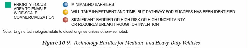
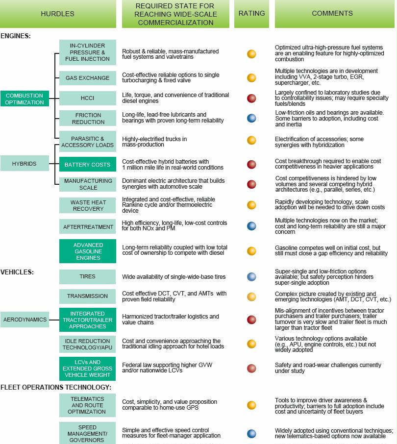
This free, 251 page document is one of the best I’ve seen on the myriad ways trucks could double their miles-per-gallon. Below are some of the main overview charts. If you don’t have the time to read this paper, the NPC Chapter 10 Heavy-duty Engines & Vehicles is just 26 pages long and explains some of the unfamiliar terms well (see their excellent chart of priorities and obstacles at the end of this post).
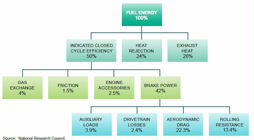
Figure 14-31. Energy Balance of a Fully Loaded Class 8 Tractor-Trailer on a Level Road at 65 mph
The first thing to know about trucks is that they are custom built to perform specific duties. What’s good for a long-haul truck might not do as much for an urban delivery truck as shown in Figure S-1. For example, all trucks and buses benefit from better engines, but long-distance trucks and coach buses don’t stop enough to benefit as much from Hybrid batteries that store braking energy as delivery and refuse trucks do, but benefit more than other trucks from aerodynamic improvements.
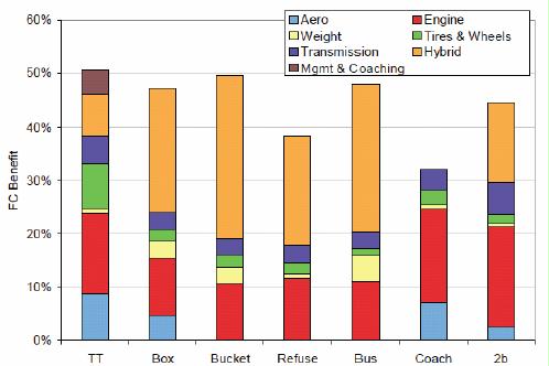
FIGURE S-1 Comparison of 2015-2020 new-vehicle potential fuel-saving technologies for seven vehicle types: tractor trailer (TT), Class 3-6 box (box), Class 3-6 bucket (bucket), Class 8 refuse (refuse), transit bus (bus), motor coach (coach), and Class 2b pickups and vans (2b). Optimal driver management and coaching would also help but this has never been quantified.
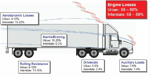
FIGURE 2-7 Energy “loss” range of vehicle attributes as impacted by duty cycle, on a level road
According to the Transportation Energy Data Book, trucks move over 8.7 billion tons of freight annually in the United States, accounting for more than two-thirds of national freight transport. There are over 8 million Class 3–8 trucks on the road, according to the American Trucking Association. A significant share of trucking companies are small businesses, with 96% operating fewer than 20 trucks and nearly 88% operating six trucks or less. Consequently, the trucking industry is a highly fragmented industry, resulting in intense competition and low profit margins.
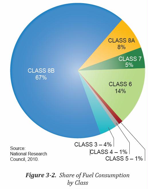
Class 7 & 8 trucks account for over 4.5 million units. These trucks represent heavy working trucks consuming typically 6,000–8,000 gallons of fuel per year for Class 7 and 10,000–13,000 gallons of fuel per year for Class 8a. Class 8b trucks are typically long-haul trucks weighing more than 33,000 pounds that have one or more trailers for flatbed, van, refrigerated, and liquid bulk. Class 7 represents some 200,000 vehicles while Classes 8a and 8b consist of 430,000 and 1,720,000, respectively. These trucks consume typically 19,000–27,000 gallons of fuel per year and account for more than 50% of the total freight tonnage moved by trucks.
The Class 8 truck market is 98% controlled by 6 brands owned by 4 companies: Freightliner, International, Peterbilt, Kenworth, Volvo, and Mack. Many of them also make Class 3-6 trucks and buses. These companies either develop their own engine platforms or buy them from independent engine manufacturers, dominated by a small number of players: Cummins, Detroit Diesel, Navistar, and Volvo Powertrain, with GM holding a key position in the Class 3-6 truck space.
TABLE S-1 Fuel Consumption Reduction Potential for Power Train Technologies
Diesel engines: 15 to 21%
Gasoline engines: Up to 24%
Diesel over gasoline engines: 6 to 24%
Improved transmissions: 4 to 8%
Hybrid power trains: 5 to 50%
TABLE S-2 Fuel Consumption Reduction Potential for Vehicle Technologies
Aerodynamics: 3 to 15%
Auxiliary loads: 1 to 2.5%
Rolling resistance (tires): 4.5 to 9%
Mass (weight) reduction: 2 to 5%
Idle reduction: 5 to 9%
Intelligent vehicle: 8 to 15%
TABLE S-3 Overall Fuel Consumption Reduction Potential for Typical New Vehicles, 2015-2020
51% Tractor-trailer
47% Class 6 box truck
50% Class 6 bucket truck
45% Class 2b pickup
38% Refuse truck
48% Transit bus
32% Motor coach
| Class |
Applications |
Gross Wt Range (lb) |
| 1c |
Cars only |
3200-6000 |
| 1t |
Minivans, small SUVs, small pick-ups |
4000-6000 |
| 2a |
Large SUVs, standard pick-ups |
6001-8500 |
| 2b |
Large pick-ups, Utility Van, Multi-porpose, Mini-bus, Step Van |
8501-10000 |
| 3 |
Utility Van, Multi-purpose, Minibus, Step Van |
10001-14000 |
| 4 |
City Delivery, Parcel Delivery, Large Walk-in, Bucket, Landscaping |
14001-16000 |
| 5 |
City Delivery, Parcel Delivery, Large Walk-in, Bucket |
16001-19500 |
| 6 |
City Delivery, School Bus, Large Walk-in, Bucket |
19501-26000 |
| 7 |
Furniture, refuse, concrete, tow, fire engine, tractor-trailer |
26001-33000 |
| 8a |
Dump, refuse, concrete, furniture, tow, fire engine, city bus |
33001-80000 |
| 8b |
Tractor-trailer, Bulk Tanker, Flat bed |
33001-80000 |
The 6 miles per gallon (mpg) fuel economy of a line-haul truck seems paltry compared to the 40 mpg of a car. But when the fuel used to move cargo weight is considered, the big truck looks pretty good. A large class 8 truck carrying 42,000-pounds of goods at 6 mpg of fuel economy is carrying 126 tons of freight per mile, or 126 ton mpg. But a car with 500 pounds of people and luggage is only getting 10 ton mpg, less than 10% of the large truck.
So when diesel and gasoline are rationed, someone needs to figure out situations where it makes more sense to delivery food and other essential items to homes rather than having each household drive to stores.
Cl
|
Gross Weight Range (lb) |
Empty Weight Range (lb) |
Typical Payload (cargo) weight |
Payload capacity Max (% of Empty) |
2006 Unit sales volume |
Typical mpg range 2007 |
Avg ton mpg |
| 1c |
3200-6000 |
2400-5000 |
250-1000 |
10-20 |
7,781,000 |
25-33 |
15 |
| 1t |
4000-6000 |
3200-4500 |
250-1500 |
8-33 |
6,148,000 |
20-25 |
17 |
| 2a |
6001-8500 |
4500-6000 |
250-2500 |
6-40 |
3,020,000 |
20-21 |
26 |
| 2b |
8501-10000 |
5000-6300 |
3700 |
60 |
545,000 |
10-15 |
26 |
| 3 |
10001-14000 |
7650-8750 |
5250 |
60 |
137,000 |
8-13 |
30 |
| 4 |
14001-16000 |
7650-8750 |
7250 |
80 |
48,000 |
7-12 |
42 |
| 5 |
16001-19500 |
9500-10800 |
8700 |
80 |
41,000 |
6-12 |
39 |
| 6 |
19501-26000 |
11500-14500 |
11500 |
80 |
65,000 |
5-12 |
49 |
| 7 |
26001-33000 |
11500-14500 |
18500 |
125 |
82,411 |
4-8 |
55 |
| 8a |
33001-80000 |
20000-34000 |
20000-50000 |
100-150 |
45,600 |
2.5-6 |
115 |
| 8b |
33001-80000 |
23500-80000 |
40000-54000 |
125-200 |
182,395 |
4-7.5 |
155 |
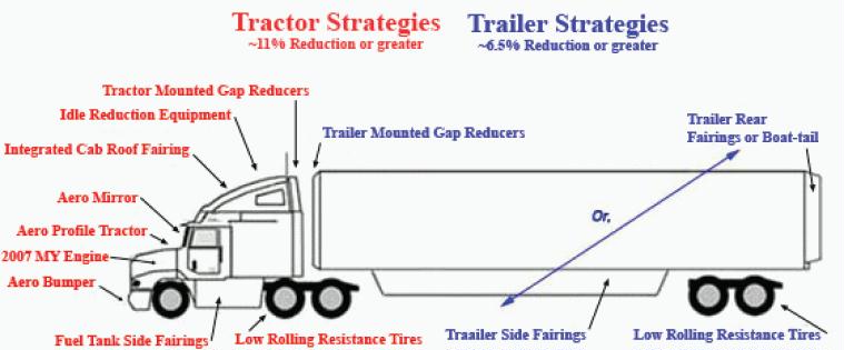
FIGURE 3-7 Some aerodynamic technologies
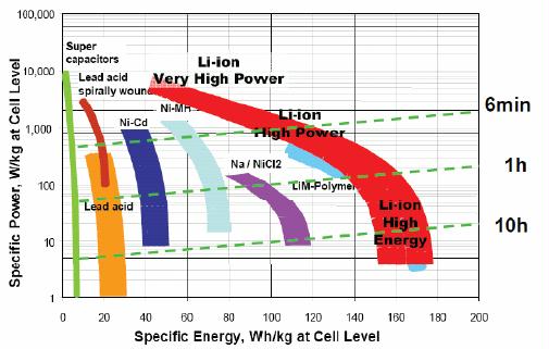
FIGURE 4-15 Battery type versus specific power and energy. SOURCE: Kalhammer et al. (2007).
It’s easy to see why lithium ion batteries are winning out over other battery technologies — they have both higher power (I want it NOW) and higher energy (long distance for hours) and weigh less. But li-ion perform poorly, and don’t achieve their optimal driving range under 32 F and over 95 F. Hot temperatures also shortens li-ion battery life.
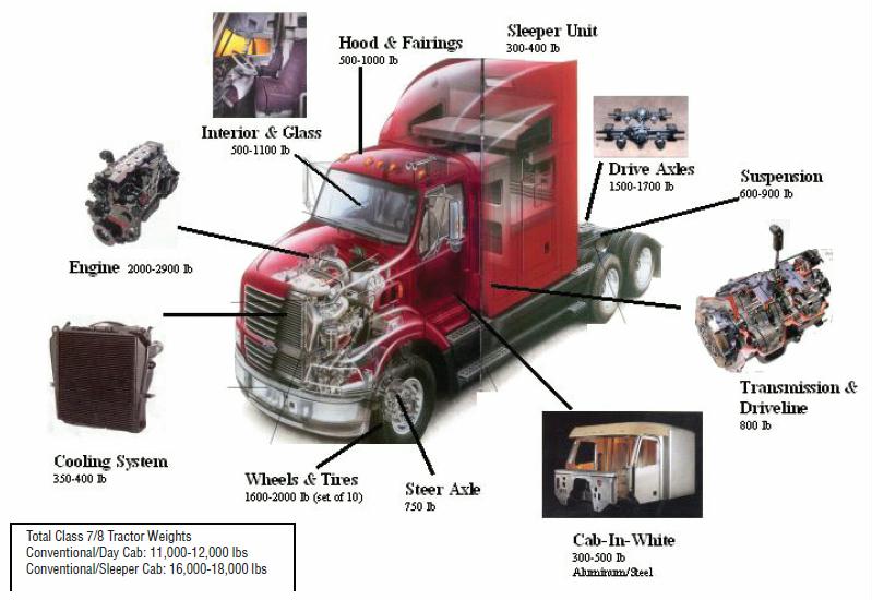
| % of weight |
lbs |
Major |
Description |
| 24 |
4080 |
Powertrain |
Engine and cooling system, transmission, accessories |
| 19 |
3230 |
Truck body structure |
Cab-in-white, sleeper unit, hood & fairings, Interior & glass |
| 18 |
3060 |
Misc Accessories/systems |
Batteries, fuel system, exhaust hardware |
| 17 |
2890 |
Drivetrain & Suspension |
Drive axles, steer axle, suspension system |
| 12 |
2040 |
Chassis / Frame |
Frame rails & crossmembers, Fifth wheel and brackets |
| 10 |
1700 |
Wheels and Tires |
Set of 10 aluminum wheel + tire |
Figure 5-32 Weight distribution of major component categories in Class 8 tractors. SOURCE: Smith and Eberle (2003).
Potential for Lightweighting Trucks
Class 8 trucks, per 1,000 pounds lighter, get up to 1% better fuel efficiency on level ground, 1.6% better in stop and go traffic, and up to 2.4% better going uphill (Table 5-16, not shown).
Trucks, trailers, and buses are benefiting from greater use of lightweight materials and structures. Components already making use of aluminum include the cab structure, wheels, fifth wheel, bellhousing, and more (see Table 5-17). Aluminum composite panels have been introduced on trailers, and the use of wood in trailers is diminishing. The barrier to additional use of aluminum or carbon composites is primarily cost effectiveness, with carbon fiber composites, for example, costing several times more per unit mass than aluminum. Some technical and cost-effectiveness issues with carbon composites and have been studied in DOE programs with industry (Rini, 2005).
While progress is being made in weight reduction through materials and design, certain weight-adding components have been necessary. Emissions control components are adding roughly 400 lb, and aerodynamic devices another 200 lb, but are deemed a positive tradeoff with aerodynamic drag reduction. Similarly, the weight addition from efficiency technologies such as waste heat recovery are projected to provide net benefits. In hybrid applications, batteries and other hybrid components add 300 to 1000 lb for trucks and even more in bus applications.
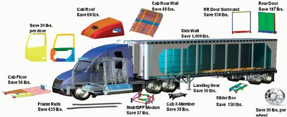
FIGURE 5-38 Weight reduction opportunities with aluminum.
| Technologies |
Class 8 |
Class 3-7 |
Refuse Truck |
| Trailer aerodynamics |
X |
|
|
| Cab aerodynamics |
X |
X |
|
| Tires and Wheels |
X |
X |
X |
| Weight reduction |
X |
X |
X |
| Transmission & driveline |
X |
X |
X |
| Accessory electrification |
X |
X |
|
| Overnight idle reduction |
X |
|
|
| Idle reduction |
X |
X |
|
| Engine efficiency |
X |
X |
X |
| Waste heat recapture |
X |
|
|
| Hybridization |
X |
X |
X |
| Dieselization (from gasoline) |
|
X |
|
| TABLE 6-1 Technologies and Vehicle Classes Likely to See Benefits |
|
|
|
|
|
|
|
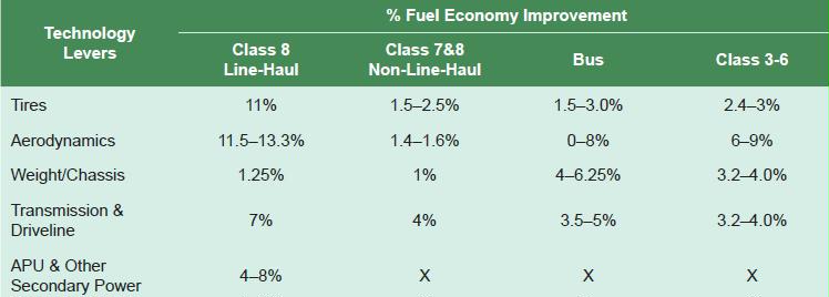
| Fuel Consumption reduction % |
|
|
|
| Engine |
20 |
11-14 |
14 |
| Aerodynamics |
11.5 |
6 |
0 |
| Rolling Resistance |
11 |
3 |
1.5 |
| Transmission & driveline |
7 |
4 |
4 |
| Hybrids |
10 |
30-40 |
35 |
| Weight |
1.25 |
4 |
1 |
| TABLE 6-2 Fuel Consumption Reduction (percentage) by Application and Vehicle Type |
|
|
|
Tractors designed with aerodynamics in mind have been on the market for almost 30 years. A relatively wide range of aero-related improvements have been implemented on modern truck tractors, which has substantially improved their fuel economy. Figure 10-7 shows a summary of aerodynamic
More on aerodynamic design
[I think that this will be less of an issue as roads crumble and long-haul trucks can’t go fast, and hopefully railroads will be carrying a larger share of long-distance freight since they’ll have plenty of room once a great depression hits and less goods are traveling]
Some measures, such as roof fairings and deflectors, have been widely adopted throughout the trucking industry, while others are less prevalent. Improvements in fuel economy on the order of 10% have already been documented, owing to a combination of tractor aerodynamic measures.
The prospect of high fuel prices has renewed industry interest in active aerodynamics. Examples of active aerodynamic systems include the following: Grille shutters to close off the grille when active y engine cooling is not needed.
Active ride height control to lower the tractor and trailer at highway speeds. This technology lowers the total vehicle by 0.75 to 1.0 inch, which reduced overall form drag by reducing frontal area. Deployable mirrors or in-cabin vision systems to take over mirror functionality at highway speeds when the mirrors would be stowed for improved aerodynamics. Current safety regulations, which require fixed mirrors, prevent this technology from being deployed.
Trailer side skirts, mounted under the trailer and deflecting airflow from sweeping the trailer underside, have been shown to have a substantial aerodynamic effect. Fuel economy improvements of between 3.8 and 5.2% have been reported for such devices. However, while aerodynamically compelling, these features cause a wide variety of problems for fleet operators. Service, inspection, tire storage, and tire maintenance are all hindered by lack of easy access to the trailer underside. And skirts are prone to damage and breakage in the harsh environment where trailers must operate. These include the conditions at work sites, around fork trucks, in ice and snow, at steep loading docks, and similar conditions.
The rear of the trailer can be optimized for low drag using a “boat-tail” or similar device to reduce the massive separation bubble that follows the trailer back surface. Improvements in fuel economy ranging from 2.9 to 5.0% have been reported. As with side skirts, however, such devices have been resisted by the truck-buying fleets due to practical concerns.
Generally speaking, aerodynamic improvements to trailers have been slower and less noticeable than those on the tractor. This is largely due to the different ownership models of tractors versus trailers. Tractors are specified meticulously, and represent a major investment for their owners. A trailer costs much less, and is often seen as an interchangeable commodity with substantial cost pressure. Further, trailers are far more numerous than tractors, by a factor of 4:1 in a typical fleet. Many trailers are therefore sitting idle at any given time; the net result is a much longer payback time for investments in trailer efficiency. And finally, in some cases, the trailer is not owned by the same entity that owns the tractor and pays for the fuel. This misalignment of incentives is a hurdle to more aggressive implementation of trailer aerodynamic measures.
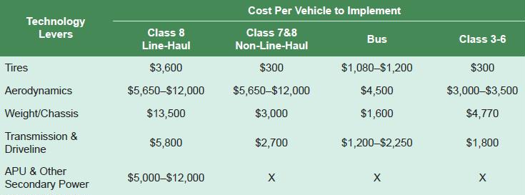
Tires
Rolling resistance accounts for roughly one-third of the power required to move a heavy truck over a level road at highway speeds. Rolling resistance comes primarily from inelastic deformation of the tire as it rotates. This deformation is a complex function of the load level, tire materials, tire and tread design, inflation levels, and the road surface itself. Generally speaking, the resistive force is proportional to the weight of the vehicle. In terms of energy consumption, the impact of rolling resistance is directly proportional to vehicle speed. Opportunities for reducing tire resistance are highly dependent on application as discussed below.
Wide-Base Single Tires. In Class 8 line-haul applications, operation is exclusively on-road and most time is spent at higher speeds, which provides several opportunities for optimization. The most significant development is the so-called “New-Generation Wide-Base Single” (NGWBS) tire, which employs a wider tread to replace two traditional truck tires with a single tire. Studies show fuel economy improvements in the range of 5 to 10% for the use of NGWBS tires in line-haul applications. These gains must be traded off against several downsides of such tires, including an added capital cost of around $3,600 per vehicle, and a perception of reduced safety.
NGWBS tires are not the only means to reduce tire rolling resistance. Proper inflation and alignment can also contribute to better fuel economy. Maintenance of proper inflation levels can be improved by tire pressure monitoring, and in some cases by the use of nitrogen gas in the place of air. The total effect of such changes is around 1.5 to 3%. However, with the exception of pressure monitoring, these modifications are very low-cost options, requiring only basic service and attention to the vehicle. The cost of such activity is estimated at only around $300 per vehicle, for both Class 3-6 vehicles and vocational Class 8 trucks. These improvements are particularly relevant for non-line-haul vehicles, where NGWBS tires are often not an option.
Vehicle Weight
Vehicle weight is a significant factor in fuel economy and puts stress on roads causing billions of dollars of needed repairs every year. It has an impact on the power required to accelerate, and the power dissipated in the form of braking.
Vehicle weight also impacts such factors as rolling resistance and transmission performance, so that weight is an ever-present factor in truck fuel economy. It is most prevalent for vehicles with frequent changes in speed, which tends to dissipate more energy braking than constant-speed
The benefit of lower weight has been studied for a wide class of vehicle types, with varying results.
For line-haul trucks over level terrain, a benefit of between 0.4 and 1.0% in fuel economy is reported per 1,000 pounds of weight reduction. The benefit improves to 1.5– 2.0% for uphill climbing routes, where more energy is invested in pulling the weight of the vehicle to higher elevation. Data on other types of vehicle are less consistent, with results generally in the low single-digits of fuel economy improvement, depending on vehicle class and duty cycle.
All-electric truck battery weight
The battery weight for a class 8 truck is roughly 55,000 lbs and the max cargo weight is 59,000 lbs, so clearly it is impossible to electrify class 7-8 trucks unless battery energy density increases at least 10-fold.
All-electric truck batteries weight about 22 kg per kwh, and a typical class 3-6 battery is 80 kWh, so 1760 kg or 3880 lbs, and that will not only lower the distance the truck can go, but the amount of cargo weight it can carry.
Idling. Line-haul truck engines spend many hours idling in a given 24-hour period. Engine idling is used for a variety of functions when the truck is stationary, such as powering air-conditioners, providing electrical power for TVs, laptops, kitchenettes, etc., providing cabin heat in cold temperatures, and maintaining engine temperature. Though an idling diesel engine is not efficient, it is a simple and easy way to provide these functions to the typical long-haul trucker.
Reducing a single truck’s idling time by 15 minutes per day can save hundreds of dollars per year in fuel costs.
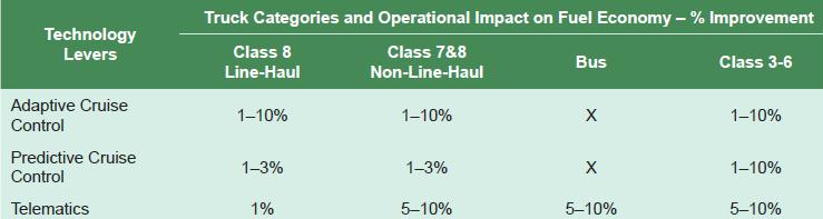
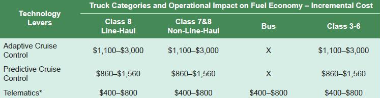
Telematic systems provide information to fleet managers and truckers with the primary objective of improving fleet efficiencies and fuel economy. Idle reduction and route management are examples of telematic applications. Idle time can be reduced using telematics in multiple ways. For example, with real-time knowledge of truck location and route traffic, a fleet manager can direct drivers to nearby trucks stops with hotel-load capacity or similar idle-elimination capabilities. By using telematic technologies to keep trucks on-route, fewer loads are delayed through unplanned route changes, and more trucks arrive at their destination on-time without overnight stops. These advantages can have a sizeable impact on fleet fuel economy.
Telematic technologies are also instrumental in route management. This includes both planning of routes based on past history of truck routes and active real-time management of truck route following. A study conducted for a report by TIAX in 2009 found that route optimization software was able to reduce pick-up and delivery fleet mileage between 5 and 10% per year. For regional and line-haul fleets, which spend relatively less time in traffic, the fuel savings potential was approximately 1% per year according to the NRC.