Preface. Jason Bradford is amazing: He taught ecology for a few years at Washington University in St. Louis, worked for the Center for Conservation and Sustainable Development at the Missouri Botanical Garden, and co-founded the Andes Biodiversity and Ecosystem Research Group (ABERG). After joining with the Post Carbon Institute in 2004 he shifted from academia to sustainable agriculture, had six months of training with Ecology Action (aka GrowBiointensive) in Willits, California, started the Willits Economic LocaLization and hosted The Reality Report radio show on KZYX in Mendocino County. In 2009 he moved to Corvallis, Oregon, as one of the founders of Farmland LP, a farmland management fund implementing organic and mixed crop and livestock systems. He now lives with his family outside of Corvallis on an organic farm.
Below is the Introduction of his book “The Future is Rural” followed by an older piece he wrote back in 2009.
Eshel G (2021) Small-scale integrated farming systems can abate continental-scale nutrient leakage. PLOS Biology. Eshel calculated how adopting nitrogen-sparing agriculture in the USA could feed the country nutritiously and reduce nitrogen leakage into water supplies. He proposes to shift to small, mixed agricultural farms with the core 1.43-hectares an intensive cattle facility from which manure production supports crops for humans as well as livestock fodder.
Today’s economic globalization is the most extreme case of complex social organization in history—and the energetic and material basis for this complexity is waning. Not only are concentrated raw resources becoming rarer, but previous investments in infrastructure (for example, ports) are in the process of decay and facing accelerating threats from climate change and social disruptions. 2 The collapse of complex societies is a historically common occurrence,3 but what we are facing now is at an unprecedented scale. Contrary to the forecasts of most demographers, urbanization will reverse course as globalization unwinds during the 21st century. The eventual decline in fossil hydrocarbon flows, and the inability of renewables to fully substitute, will create a deficiency of energy to power bloated urban agglomerations and require a shift of human populations back to the countryside. 4 In short, the future is rural.
Given the drastic changes that are unfolding, this report has four main aims:
Understand how we got to a highly urbanized, globalized society and why a more rural, relocalized society is inevitable.
Provide a framework (sustainability and resilience science) for how to think about our predicament and the changes that will need to occur.
Review the most salient aspects of agronomy, soil science, and local food systems, including some of the schools of thought that are adapted to what’s in store.
Offer a strategy and tactics to foster the transformation to a local, sustainable, resilient food system.
This report reviews society’s energy situation; explores the consequences for producing, transporting, storing, and consuming food; and provides essential information and potentially helpful advice to those working on reform and adaptation. It presents a difficult message. Our food system is at great risk from a problem most are not yet aware of, i.e., energy decline. Because the problem is energy, we can’t rely on just-in-time innovative technology, brilliant experts, and faceless farmers in some distant lands to deal with it. Instead, we must face the prospect that many of us will need to be more responsible for food security. People in highly urbanized and globally integrated countries like the U.S. will need to reruralize and relocalize human settlement and subsistence patterns over the coming decades to adapt to both the end of cheaply available fossil fuels and climate change.
These trends will require people to change the way they go about their lives, and the way their communities go about business. There is no more business as usual. The point is not to give you some sort of simple list of “50 things you should do to save the planet” or “the top 10 ways to grow food locally.” Instead, this report provides the broad context, key concepts, useful information, and ways of thinking that will help you and those around you understand and adapt to the coming changes.
To help digest the diverse material, the report is divided into five sections plus a set of concluding thoughts:
Part One sets the broad context of how fossil hydrocarbons—coal, oil and natural gas—transformed civilization, how their overuse has us in a bind, and why renewable energy systems will fall short of most expectations.
Part Two presents ways to think about how the world works from disciplines such as ecology, and highlights the difference between more prevalent, but outdated, mental models.
Part Three reviews basic science on soils and agronomy, and introduces historical ways people have fed themselves.
Part Four outlines some modern schools of thought on agrarian ways of living without fossil fuels.
Part Five brings the knowledge contained in the report to bear on strategies and tactics to navigate the future. Although the report is written for a U.S. audience, much of the content is more widely applicable.
During the process of writing this report, thought leaders and practitioners were interviewed to capture their perspectives on some of the key questions that arise from considering the decline of fossil fuels, consequences for the food system, and how people can adapt. Excerpts from those interviews are given in the Appendix section “Other Voices,” and several of their quotes are inserted throughout the main text.
Globalization has become a culture, and the prospect of losing this culture is unsettling. Much good has arisen from the integration and movements of people and materials that have occurred in the era of globalization. But we will soon be forced to face the consequences of unsustainable levels of consumption and severe disruption of the biosphere. For the relatively wealthy, these consequences have been hidden by tools of finance and resources flows to power centers, while people with fewer means have been trampled in the process of assimilation. In the U.S., our food system is culturally bankrupt, mirroring and contributing to crises of health and the environment. We can rebuild the food system in ways that reflect energy, soil, and climate realities, seeking opportunities to recover elements of past cultures that inhabited the Earth with grace. Something new will arise, and in the evolution of what comes next, many may find what is often lacking in life today—the excitement of a profound challenge, meaning beyond the self, a deep sense of purpose, and commitment to place.
To get by on ambient energy as much as possible, we have sought alternatives to fossil fuels in every aspect of the food system we participate in. Table 1 considers each type of work done on the farm, to the fork, and back again and contrasts how fossil fuels are commonly used with the technologies we have applied.
Type of Work
Common Fossil-Fuel Inputs
Alternatives Implemented
Soil cultivation
Gasoline or diesel powered rototiller or small tractor
Low-wheel cultivator, broadfork, adze or grub hoe, rake and human labor
Soil fertility
In-organic or imported organic fertilizer
Growing of highly productive, nitrogen and biomass crop (banner fava beans), making aerobic compost piles sufficient to build soil carbon and nitrogen fertility, re-introducing micro-nutrients by importing locally generated food waste and processing in a worm bin, and application of compost teas for microbiology enhancement.
Pest and weed management
Herbicide and pesticide applications, flame weeder, tractor cultivation
Companion planting, crop rotation, crop diversity and spatial heterogeneity, beneficial predator attraction through landscape plantings, emphasis on soil and plant health, and manual removal with efficient human-scaled tools
Seed sourcing
Bulk ordering of a few varieties through centralized seed development and distribution outlets
Sourcing seeds from local supplier, developing a seed saving and local production and distribution plan using open pollinated varieties
Food distribution
Produce trucks, refrigeration, long-distance transport, eating out of season
Produce only sold locally, direct from farm or hauled to local restaurants or grocers using bicycles or electric vehicles, produce grown with year-round consumption in mind with farm delivering large quantities of food in winter months
Storage and processing at production end
Preparation of food for long distance transport, storage and retailing requiring energy intensive cooling, drying, food grade wax and packaging
Passive evaporative cooling, solar dehydrating, root cellaring and re-usable storage baskets and bags
Home and institutional storage and cooking
Natural gas, propane or electric fired stoves and ovens, electric freezers and refrigerators
Solar ovens, promotion of eating fresh and seasonal foods, home-scale evaporative cooling for summer preservation and “root cellaring” techniques for winter storage
Table 1. Feeding people requires many kinds of work and all work entails energy. In most farm operations the main energy sources are fossil fuels. By contrast, Brookside Farm uses and develops renewable energy based alternatives.
Our use of food scraps to replace exported fertility also reduces energy by diverting mass from the municipal waste stream. Solid Waste of Willits has a transfer station in town but no local disposal site. Our garbage is trucked to Sonoma County about 100 miles to the south. From there it may be sent to a rail yard and taken several hundred miles away to an out of state land fill. We are also installing a rainwater catchment and storage system that will supply about half the annual water needs to offset use of treated municipal water. The associated irrigation system will be driven by a photovoltaic system instead of the usual diesel-driven pumps on many farms.
Let me put the area of lawn from this study into a food perspective. The 128,000 square kilometers of lawns is the same as 32 million acres. A generous portion of fruits and vegetables for a person per year is 700 lbs, or about half the total weight of food consumed in a year.[xviii] Modest yields in small farms and gardens would be in the range of about 20,000 lbs per acre.[xix] Even with half the area set aside to grow compost crops each year, simple math reveals that the entire U.S. population could be fed plenty of vegetables and fruits using two thirds of the area currently in lawns.
Number of people in U.S.
300,000,000
Pounds of fruits and vegetables per person per year
700
Yield per acre in pounds
20,000
People fed per acre in production
29
Fraction of area set aside for compost crops
0.5
Compost-adjusted people fed per acre
14
Number of acres to feed population
21,000,000
Acres in lawn
32,000,000
Percent of lawn area needed
66%
Labor Compared to Hours of T.V.
For its members Brookside Farm’s role is to provide a substantial proportion of their yearly vegetable and fruit needs. Using our farming techniques, we estimate that one person working full time could grow enough produce for ten to twenty people. By contrast, an individual could grow their personal vegetable and fruit needs on a very part-time basis, probably half an hour per day, on average, working an area the size of a small home (700 sq ft in veggies and fruits plus 700 sq ft in cover crops). American’s complain that they feel cramped for time and overworked. But is this really true or just a function of addiction to a fast-paced media culture? According to Nielsen Media Research:[xx]
Preface. If peak oil did indeed happen in 2018 as the EIA world production data shows, then let’s use the oil we still have, before it is rationed, to clean up the 126,000+ sites that threaten to pollute groundwater for thousands of years as this report from the National Research Council explains. And while we’re at it, nuclear waste, which will pollute for hundreds of thousands of years.
NRC. 2013. Alternatives for Managing the Nation’s Complex Contaminated Groundwater Sites. National Research Council, National Academies Press.
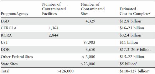
TABLE 2-6 Rough Estimate of the total number of currently known facilities or contaminated sites and estimated costs to complete
CONCLUSIONS AND RECOMMENDATIONS At least 126,000 sites across the country have been documented that have residual contamination at levels preventing them from reaching closure.
This number is likely to be an underestimate of the extent of contamination in the United States for a number of reasons. For some programs data are available only for contaminated facilities rather than individual sites, and the total does not include sites that likely exist but have not yet been identified, such as dry cleaners or small chemical-intensive businesses (e.g., electroplating, furniture refinishing). Information on cleanup costs incurred to date and estimates of future costs, as shown in Table 2-6, are highly uncertain. Despite this uncertainty, the estimated “cost to complete” of $110-$ 127 billion is likely an underestimate of future liabilities. Remaining sites include some of the most difficult to remediate sites, for which the effectiveness of planned remediation remains uncertain given their complex site conditions. Furthermore, many of the estimated costs do not fully consider the cost of long-term management of sites that will have contamination remaining in place at high levels for the foreseeable future.
Despite nearly 40 years of intensive efforts in the United States as well as in other industrialized countries worldwide, restoration of groundwater contaminated by releases of anthropogenic chemicals to a condition allowing for unlimited use and unrestricted exposure remains a significant technical and institutional challenge.
Recent estimates by the U.S. Environmental Protection Agency (EPA) indicate that expenditures for soil and groundwater cleanup at over 300,000 sites through 2033 may exceed $200 billion (not adjusted for inflation), and many of these sites have experienced groundwater impacts.
One dominant attribute of the nation’s efforts on subsurface remediation efforts has been lengthy delays between discovery of the problem and its resolution. Reasons for these extended timeframes are now well known: ineffective subsurface investigations, difficulties in characterizing the nature and extent of the problem in highly heterogeneous subsurface environments, remedial technologies that have not been capable of achieving restoration in many of these geologic settings, continued improvements in analytical detection limits leading to discovery of additional chemicals of concern, evolution of more stringent drinking water standards, and the realization that other exposure pathways, such as vapor intrusion, pose unacceptable health risks. A variety of administrative and policy factors also result in extensive delays, including, but not limited to, high regulatory personnel turnover, the difficulty in determining cost-effective remedies to meet cleanup goals, and allocation of responsibility at multiparty sites.
There is general agreement among practicing remediation professionals, however, that there is a substantial population of sites, where, due to inherent geologic complexities, restoration within the next 50 to 100 years is likely not achievable. Reaching agreement on which sites should be included in this category, and what should be done with such sites, however, has proven to be difficult. A key decision in that Road Map is determining whether or not restoration of groundwater is “likely.
Summary
The nomenclature for the phases of site cleanup and cleanup progress are inconsistent between federal agencies, between the states and federal government, and in the private sector. Partly because of these inconsistencies, members of the public and other stakeholders can and have confused the concept of “site closure” with achieving unlimited use and unrestricted exposure goals for the site, such that no further monitoring or oversight is needed. In fact, many sites thought of as “closed” and considered as “successes” will require oversight and funding for decades and in some cases hundreds of years in order to be protective.
At hundreds of thousands of hazardous waste sites across the country, groundwater contamination remains in place at levels above cleanup goals. The most problematic sites are those with potentially persistent contaminants including chlorinated solvents recalcitrant to biodegradation, and with hydrogeologic conditions characterized by large spatial heterogeneity or the presence of fractures. While there have been success stories over the past 30 years, the majority of hazardous waste sites that have been closed were relatively simple compared to the remaining caseload.
At least 126,000 sites across the country have been documented that have residual contamination at levels preventing them from reaching closure. This number is likely to be an underestimate of the extent of contamination in the United States
Significant limitations with currently available remedial technologies persist that make achievement of Maximum Contaminant Levels (MCL) throughout the aquifer unlikely at most complex groundwater sites in a time frame of 50-100 years. Furthermore, future improvements in these technologies are likely to be incremental, such that long-term monitoring and stewardship at sites with groundwater contamination should be expected.
IMPLICATIONS OF CONTAMINATION REMAINING IN PLACE
Chapter 5 discusses the potential technical, legal, economic, and other practical implications of the finding that groundwater at complex sites is unlikely to attain unlimited use and unrestricted exposure levels for many decades. First, the failure of hydraulic or physical containment systems, as well as the failure of institutional controls, could create new exposures. Second, toxicity information is regularly updated, which can alter drinking water standards, and contaminants that were previously unregulated may become so. In addition, pathways of exposure that were not previously considered can be found to be important, such as the vapor intrusion pathway. Third, treating contaminated groundwater for drinking water purposes is costly and, for some contaminants, technically challenging. Finally, leaving contamination in the subsurface may expose the landowner, property manager, or original disposer to complications that would not exist in the absence of the contamination, such as natural resource damages, trespass, and changes in land values. Thus, the risks and the technical, economic, and legal complications associated with residual contamination need to be compared to the time, cost, and feasibility involved in removing contamination outright.
New toxicological understanding and revisions to dose-response relationships will continue to be developed for existing chemicals, such as trichloroethene and tetrachloroethene, and for new chemicals of concern, such as perchlorate and perfluorinated chemicals. The implications of such evolving understanding include identification of new or revised ARARs (either more or less restrictive than existing ones), potentially leading to a determination that the existing remedy at some hazardous waste sites is no longer protective of human health and the environment.
Introduction
Since the 1970s, hundreds of billions of dollars have been invested by federal, state, and local government agencies as well as responsible parties to mitigate the human health and ecological risks posed by chemicals released to the subsurface environment. Many of the contaminants common to these hazardous waste sites, such as metals and volatile organic compounds, are known or suspected to cause cancer or adverse neurological, reproductive, or developmental conditions.
Over the past 30 years, some progress in meeting mitigation and remediation goals at hazardous waste sites has been achieved. For example, of the 1,723 sites ever listed on the National Priorities List (NPL), which are considered by the U.S. Environmental Protection Agency (EPA) to present the most significant risks, 360 have been permanently removed from the list because EPA deemed that no further response was needed to protect human health or the environment (EPA, 2012).
Seventy percent of the 3,747 hazardous waste sites regulated under the Resource Conservation and Recovery Act (RCRA) corrective action program have achieved “control of human exposure to contamination,” and 686 have been designated as “corrective action completed”. The Underground Storage Tank (UST) program also reports successes, including closure of over 1.7 million USTs since the program was initiated in 1984. The cumulative cost associated with these national efforts underscores the importance of pollution prevention and serves as a powerful incentive to reduce the discharge or release of 13 hazardous substances to the environment, particularly when a groundwater resource is threatened. Although some of the success stories described above were challenging in terms of contaminants present and underlying hydrogeology, the majority of sites that have been closed were relatively simple (e.g., shallow, localized petroleum contamination from USTs) compared to the remaining caseload.
Indeed, hundreds of thousands of sites across both state and federal programs are thought to still have contamination remaining in place at levels above those allowing for unlimited land and groundwater use and unrestricted exposure (see Chapter 2). According to its most recent assessment, EPA estimates that more than $209 billion dollars (in constant 2004 dollars) will be needed over the next 30 years to mitigate hazards at between 235,000 to 355,000 sites (EPA, 2004). This cost estimate, however, does not include continued expenditures at sites where remediation is already in progress, or where remediation has transitioned to long-term management.
It is widely agreed that long-term management will be needed at many sites for the foreseeable future, particularly for the more complex sites that have recalcitrant contaminants, large amounts of contamination, and/or subsurface conditions known to be difficult to remediate (e.g., low-permeability strata, fractured media, deep contamination).
According to the most recent annual report to Congress, the Department of Defense (DoD) currently has almost 26,000 active sites under its Installation Restoration Program where soil and groundwater remediation is either planned or under way. Of these, approximately 13,000 sites are the responsibility of the Army, the sponsor of this report. The estimated cost to complete cleanup at all DoD sites is approximately $12.8 billion. (Note that these estimates do not include sites containing unexploded ordnance.)
Complex Contaminated Sites
Although progress has been made in remediating many hazardous waste sites, there remains a sizeable population of complex sites, where restoration is likely not achievable in the next 50-100 years. Although there is no formal definition of complexity, most remediation professionals agree that attributes include a really extensive groundwater contamination, heterogeneous geology, large releases and/or source zones, multiple and/or recalcitrant contaminants, heterogeneous contaminant distribution in the subsurface, and long time frames since releases occurred.
Complexity is also directly tied to the contaminants present at hazardous waste sites, which can vary widely and include organics, metals, explosives, and radionuclides. Some of the most challenging to remediate are dense nonaqueous phase liquids (DNAPLs), including chlorinated solvents.
Each of the NRC studies has, in one form or another, recognized that in almost all cases, complete restoration of contaminated groundwater is difficult, and in a substantial fraction of contaminated sites, not likely to be achieved in less than 100 years.
Trichloroethene (TCE) and tetrachloroethene are particularly challenging to restore because of their complex contaminant distribution in the subsurface.
Three classes of contaminants that have proven very difficult to treat once released to the subsurface: metals, radionuclides, and DNAPLs, such as chlorinated solvents. The report concluded that “removing all sources of groundwater contamination, particularly DNAPLs, will be technically impracticable at many Department of Energy sites, and long-term containment systems will be necessary for these sites.”
An example of the array of challenges faced by the DoD is provided by the Anniston Army Depot, where groundwater is contaminated with chlorinated solvents (as much as 27 million pounds of TCE and inorganic compounds. TCE and other contaminants are thought to be migrating vertically and horizontally from the source areas, affecting groundwater downgradient of the base including the potable water supply to the City of Anniston, Alabama. The interim Record of Decision called for a groundwater extraction and treatment system, which has resulted in the removal of TCE in extracted water to levels below drinking water standards. Because the treatment system is not significantly reducing the extent or mobility of the groundwater contaminants in the subsurface, the current interim remedy is considered “not protective.” Therefore, additional efforts have been made to remove greater quantities of TCE from the subsurface, and no end is in sight. Modeling studies suggest that the time to reach the TCE MCL in the groundwater beneath the source areas ranges from 1,200 to 10,000 years, and that partial source removal will shorten those times to 830–7,900 years.
The Department of Defense
The DoD environmental remediation program, measured by the number of facilities, is the largest such program in the United States, and perhaps the world.
The Installation Restoration Program (IRP), which addresses toxic and radioactive wastes as well as building demolition and debris removal, is responsible for 3,486 installations containing over 29,000 contaminated sites
The Military Munitions Response Program, which focuses on unexploded ordnance and discarded military munitions, is beyond the scope of this report and is not discussed further here, although its future expenses are greater than those anticipated for the IRP.
The CERCLA program was established to address hazardous substances at abandoned or uncontrolled hazardous waste sites. Through the CERCLA program, the EPA has developed the National Priorities List (NPL). There are 1,723 facilities that have been on the NPL.
As of June 2012, 359 of the 1,723 facilities have been “deleted” from the NPL, which means the EPA has determined that no further response is required to protect human health or the environment; 1,364 remain on the NPL.
Statistics from EPA (2004) illustrate the typical complexity of hazardous waste sites at facilities on the NPL. Volatile organic compounds (VOCs) are present at 78 percent of NPL facilities, metals at 77 percent, and semivolatile organic compounds (SVOCs) at 71 percent. All three contaminant groups are found at 52 percent of NPL facilities, and two of the groups at 76 percent of facilities
RCRA Corrective Action Program Among other objectives, the Resource Conservation and Recovery Act (RCRA) governs the management of hazardous wastes at operating facilities that handle or handled hazardous waste.
Although tens of thousands of waste handlers are potentially subject to RCRA, currently EPA has authority to impose corrective action on 3,747 RCRA hazardous waste facilities in the United States
Underground Storage Tank Program In 1984, Congress recognized the unique and widespread problem posed by leaking underground storage tanks by adding Subtitle I to RCRA.
UST contaminants are typically light nonaqueous phase liquids (LNAPLs) such as petroleum hydrocarbons and fuel additives.
Responsibility for the UST program has been delegated to the states (or even local oversight agencies such as a county or a water utility with basin management programs), which set specific cleanup standards and approve specific corrective action plans and the application of particular technologies at sites. This is true even for petroleum-only USTs on military bases, a few of which have hundreds of such tanks.
At the end of 2011, there were 590,104 active tanks in the UST program
Currently, there are 87,983 leaking tanks that have contaminated surrounding soil and groundwater, the so-called “backlog.” The backlog number represents the cumulative number of confirmed releases (501,723) minus the cumulative number of completed cleanups (413,740).
Department of Energy
The DOE faces the task of cleaning up the legacy of environmental contamination from activities to develop nuclear weapons during World War II and the Cold War. Contaminants include short-lived and long-lived radioactive wastes, toxic substances such as chlorinated solvents, “mixed wastes” that include both toxic substances and radionuclides, and, at a handful of facilities, unexploded ordnance. Much like the military, a given DOE facility or installation will tend to have multiple sites where contaminants may have been spilled, disposed of, or abandoned that can be variously regulated by CERCLA, RCRA, or the UST program. T
The DOE Environmental Management program, established in 1989 to address several decades of nuclear weapons production, “is the largest in the world, originally involving two million acres at 107 sites in 35 states and some of the most dangerous materials known to man”.
Given that major DOE sites tend to be more challenging than typical DoD sites, it is not surprising that the scope of future remediation is substantial. Furthermore, because many DOE sites date back 50 years, contaminants have diffused into the subsurface matrix, considerably complicating remediation.
More recent reports suggest that about 7,000 individual release sites out of 10,645 historical release sites have been “completed,” which means at least that a remedy is in place, leaving approximately 3,650 sites remaining. In 2004, DOE estimated that almost all installations would require long-term stewardship
As of April 1995, over 3,000 contaminated sites on 700 facilities, distributed among 17 non-DoD and non-DOE federal agencies, were potentially in need of remediation. The Department of Interior (DOI), Department of Agriculture (USDA), and National Aeronautics and Space Administration (NASA) together account for about 70 percent of the civilian federal facilities reported to EPA as potentially needing remediation (EPA, 2004). EPA estimates that many more sites have not yet been reported, including an estimated 8,000 to 31,000 abandoned mine sites, most of which are on federal lands, although the fraction of these that are impacting groundwater quality is not reported. The Government Accountability Office (GAO) (2008) determined that there were at least 33,000 abandoned hardrock mine sites in the 12 western states and Alaska that had degraded the environment by contaminating surface water and groundwater or leaving arsenic-contaminated tailings piles.
State Sites
A broad spectrum of sites is managed by states, local jurisdictions, and private parties, and thus are not part of the CERCLA, RCRA, or UST programs. These types of sites can vary in size and complexity, ranging from sites similar to those at facilities listed on the NPL to small sites with low levels of contamination.
States typically define Brownfields sites as industrial or commercial facilities that are abandoned or underutilized due to environmental contamination or fear of contamination. EPA (2004) postulated that only 10 to 15 percent of the estimated one-half to one million Brownfields sites have been identified.
As of 2000, 23,000 state sites had been identified as needing further attention that had not yet been targeted for remediation (EPA, 2004). The same study estimated that 127,000 additional sites would be identified by 2030. Dry Cleaner Sites Active and particularly former dry cleaner sites present a unique problem in hazardous waste management because of their ubiquitous nature in urban settings, the carcinogenic contaminants used in the dry cleaning process (primarily the chlorinated solvent PCE, although other solvents have been used), and the potential for the contamination to reach receptors via the drinking water and indoor air (vapor intrusion) exposure pathways. Depending on the size and extent of contamination, dry cleaner sites may be remediated under one or more state or federal programs such as RCRA, CERCLA, or state mandated or voluntary programs discussed previously, and thus the total estimates of dry cleaner sites are not listed separately in
In 2004, there were an estimated 30,000 commercial, 325 industrial, and 100 coin-operated active dry cleaners in the United States (EPA, 2004). Despite their smaller numbers, industrial dry cleaners produce the majority of the estimated gallons of hazardous waste from these facilities (EPA, 2004). As of 2010, the number of dry cleaners has grown, with an estimated 36,000 active dry cleaner facilities in the United States—of which about 75 percent (27,000 dry cleaners) have soil and groundwater contamination (SCRD, 2010b). In addition to active sites, dry cleaners that have moved or gone out of business—i.e., inactive sites—also have the potential for contamination. Unfortunately, significant uncertainty surrounds estimates of the number of inactive dry cleaner sites and the extent of contamination at these sites. Complicating factors include the fact that (1) older dry cleaners used solvents less efficiently than younger dry cleaners thus enhancing the amount of potential contamination and (2) dry cleaners that have moved or were in business for long amounts of time tend to employ different cleaning methods throughout their lifetime. EPA (2004) documented at least 9,000 inactive dry cleaner sites, although this number does not include data on dry cleaners that closed prior to 1960. There are no data on how many of these documented inactive dry cleaner sites may have been remediated over the years. EPA estimated that there could be as many as 90,000 inactive dry cleaner sites in the United States.
Department of Defense The Installation Restoration Program reports that it has spent approximately $31 billion through FY 2010, and estimates for “cost to complete” exceed $12 billion
Implementation costs for the CERCLA program are difficult to obtain because most remedies are implemented by private, nongovernmental PRPs and generally there is no requirement for these PRPs to report actual implementation costs.
EPA (2004) estimated that the cost for addressing the 456 facilities that have not begun remedial action is $16-$23 billion.
A more recent report from the GAO (2009) suggests that individual site remediation costs have increased over time (in constant dollars) because a higher percentage of the remaining NPL facilities are larger and more complex (i.e., “megasites”) than those addressed in the past. Additionally, GAO (2009) found that the percentage of NPL facilities without responsible parties to fund cleanups may be increasing. When no PRP can be identified, the cost for Superfund remediation is shared by the states and the Superfund Trust Fund. The Superfund Trust Fund has enjoyed a relatively stable budget—e.g., $1.25 billion, $1.27 billion, and $1.27 billion for FY 2009, 2010, and 2011, 8 respectively—although recent budget proposals seek to reduce these levels. States contribute as much as 50 percent of the construction and operation costs for certain CERCLA actions in their state. After ten years of remedial actions at such NPL facilities, states become fully responsible for continuing long-term remedial actions.
In 2004, EPA estimated that remediation of the remaining RCRA sites will cost between $31 billion and $58 billion, or an average of $11.4 million per facility
Underground Storage Tank Program
There is limited information available to determine costs already incurred in the UST program. EPA (2004) estimated that the cost to close all leaking UST (LUST) sites could reach $12-$19 billion or an average of $125,000 to remediate each release site (this includes site investigations, feasibility studies, and treatment/disposal of soil and groundwater). Based on this estimate of $125,000 per site, the Committee calculated that remediating the 87,983 backlogged releases would require $11 billion. The presence of the recalcitrant former fuel additive methyl tert-butyl ether (MTBE) and its daughter product and co-additive tert-butyl alcohol could increase the cost per site. Most UST cleanup costs are paid by property owners, state and local governments, and special trust funds based on dedicated taxes, such as fuel taxes. Department of Energy
The Department’s FY 2011 report to Congress, which shows that DOE’s anticipated cost to complete remediation of soil and groundwater contamination ranges from $17.3 to $20.9 billion. The program is dominated by a small number of mega-facilities, including Hanford (WA), Idaho National Labs, Savannah River (SC), Los Alamos National Labs (NM), and the Nevada Test Site. Given that the cost to complete soil and groundwater remediation at these five facilities alone ranges from $16.4 to $19.9 billion (DOE, 2011), the Committee believes that the DOE’s anticipated cost-to-complete figure is likely an underestimate of the Agency’s financial burden; the number does not include newly discovered releases or the cost of long-term management at all sites where waste remains in the subsurface. Data on long-term stewardship costs, including the expense of operating and maintaining engineering controls, enforcing institutional controls, and monitoring, are not consolidated but are likely to be substantial and ongoing.
Stewardship costs for just the five facilities managed by the National Nuclear Security Administration (Lawrence Livermore National Laboratory, CA, Livermore’s Site 300, Pantex, TX, Sandia National Laboratories, NM, and the Kansas City Plant, MO) total about $45 million per year (DOE, 2012c).
Other Federal Sites EPA (2004) reports that there is a $15-$22 billion estimated cost to address at least 3,000 contaminated areas on 700 civilian federal facilities, based on estimates from various reports from DOI, USDA, and NASA. States EPA (2004) estimated that states and private parties together have spent about $1 billion per year on remediation, addressing about 5,000 sites annually under mandatory and voluntary state programs. If remediation were continued at this rate, 150,000 sites would be completed over 30 years, at a cost of approximately $30 billion (or $20,000 per site). IMPACTS TO
DRINKING WATER SUPPLIES
The Committee sought information both on the number of hazardous waste sites that impact a drinking water aquifer—that is, pose a substantial near-term risk to public water supply systems that use groundwater as a source. Unfortunately, program-specific information on water supply impacts was generally not available. Therefore, the Committee also sought other evidence related to the effects of hazardous waste disposal on the nation’s drinking water aquifers.
Despite the existence of several NPL and DoD facilities that are known sources of contamination to public or domestic wells (e.g., the San Fernando and San Gabriel basins in Los Angeles County), there is little aggregated information about the number of CERCLA, RCRA, DoD, DOE, UST, or other sites that directly impact drinking water supply systems. None of the programs reviewed in this chapter specifically compiles information on the number of sites currently adversely affecting a drinking water aquifer. However, the Committee was able to obtain information relevant to the groundwater impacts from some programs, i.e. the DoD. The Army informed the Committee that public water supplies are threatened at 18 Army installations
Also, private drinking water wells are known to be affected at 23 installations. A preliminary assessment in 1997 showed that 29 Army installations may possibly overlie one or more sole source aquifers. Some of the best known are Camp Lejeune Marine Corps Base (NC), Otis Air National Guard Base (MA), and the Bethpage Naval Weapons Industrial Reserve Plant (NY).
CERCLA. Each individual remedial investigation/feasibility study (RI/FS) and Record of Decision (ROD) should state whether a drinking water aquifer is affected, although this information has not been compiled. Canter and Sabatini (1994) reviewed the RODs for 450 facilities on the NPL. Their investigation revealed that 49 of the RODs (11 percent) indicated that contamination of public water supply systems had occurred. “A significant number” of RODs also noted potential threats to public supply wells. Additionally, the authors note that undeveloped aquifers have also been contaminated, which prevents or limits the unrestricted use (i.e., without treatment) of these resources as a future water supply.
The EPA also compiles information about remedies implemented within Superfund. EPA (2007) reported that out of 1,072 facilities that have a groundwater remedy, 106 specifically have a water supply remedy, by which we inferred direct treatment of the water to allow potable use or switching to an alternative water supply. This suggests that 10 percent of NPL facilities adversely affect or significantly threaten drinking water supply systems.
RCRA. Of the 1,968 highest priority RCRA Corrective Action facilities, EPA (2008) reported that there is “unacceptable migration of contaminated groundwater” at 77 facilities. Also, 17,042 drinking water aquifers have a RCRA facility within five miles, but without additional information, it is impossible to know if these facilities are actually affecting the water sources.
UST. In 2000, 35 states reported USTs as the number one threat to groundwater quality (and thus indirectly to drinking water). However, more specific information on the number of leaking USTs currently impacting a drinking water aquifer is not available. Other Evidence That Hazardous Waste Sites Affect Water Supplies The U.S. Geological Survey (USGS) has compiled large data sets over the past 20 years regarding the prevalence of VOCs in waters derived from domestic (private) and public wells. VOCs include solvents, trihalomethanes (some of which are solvents [e.g., chloroform], but may also arise from chlorination of drinking water), refrigerants, organic synthesis compounds (e.g., vinyl chloride), gasoline hydrocarbons, fumigants, and gasoline oxygenates. Because many (but not all) of these compounds may arise from hazardous waste sites, the USGS studies provide further insight into the extent to which anthropogenic activities contaminate groundwater supplies
Zogorski et al. (2006) summarized the presence of VOCs in groundwater, private domestic wells, and public supply wells from sampling sites throughout the United States. Using a threshold level of 0.2 µg/L—much lower than current EPA drinking water standards for individual VOCs (see Table 3-1)—14 percent of domestic wells and 26 percent of public wells had one or more VOCs present. The detection frequencies of individual VOCs in domestic wells were two to ten times higher when a threshold of 0.02 µg/L was used (see Figures 2-2 and 2-3). In public supply wells, PCE was detected above the 0.2 µg/L threshold in 5.3 percent of the samples and TCE in 4.3 percent of the samples. The total percentage of public supply wells with either PCE or TCE (or both) above the 0.2 µg/L threshold is 7.3
FIGURE 2-2 Detection frequencies in domestic well samples for 15 most frequently detected VOCs at levels of 0.2 and 0.02 mg/L. SOURCE: Zogorski et al. (2006) with illustration provided by USGS National Water Quality Assessment program. Figure 2-2 Chloroform Methyl tert-butyl ether (MTBE) Perchloroethene (PCE) Bromoform Dibromochloromethane Trichloroethene (TCE) Bromodichloromethane 1,1,1-Trichloroethane (TCA) 1,1-Dichloroethane (1,1-DCA) Dichlorodifluoromethane (CFC-12) cis-1,2-Dichloroethene (cis-1,2-DCE) 1,1-Dichloroethene (1,1-DCE) Trichlorofluoromethane (CFC-11) trans-1,2-Dichloroethene (trans-1,2-DCE) Toluene
FIGURE 2-3 The 15 most frequently detected VOCs in public supply wells. SOURCE: Zogorski et al. (2006) with illustration provided by USGS National Wa ter Quality Assessment program.Figure
Further analysis of domestic wells by DeSimone et al. (2009) showed that organic contaminants were detected in 60 percent of 2,100 sampled wells. Wells were sampled in 48 states in parts of 30 regionally extensive aquifers used for water supply. Aquifers were randomly selected for sampling and there was no prior knowledge of contamination.
Of 30 regionally extensive aquifers used for water supply. Aquifers were randomly selected for sampling and there was no prior knowledge of contamination.
Toccalino and Hopple (2010) and Toccalino et al. (2010) focused on 932 public supply wells across the United States. The public wells sampled in this study represent less than 1 percent of all groundwater that feeds the nation’s public water systems. The samples, however, were widely distributed nationally and were randomly selected to represent typical aquifer conditions. Overall, 60 percent of public wells contained one or more VOCs at a concentration of = 0.02 µg/L, and 35 percent of public wells contained one or more VOCs at a concentration of = 0.2 µg/L.
Overall detection frequencies for individual compounds included 23 percent for PCE, 15 percent for TCE, 14 percent for MTBE, and 12 percent for 1,1,1-TCA (see Figure 2-5). PCE and TCE exceeded the MCL in approximately 1 percent of the public wells sampled.
PERCENT FIGURE 2-4 VOCs (in black) and pesticides (in white) detected in more than 1 percent of domestic wells at a level of 0.02 µg/L.
FIGURE 2-5 VOCs and pesticides with detection frequencies of 1 percent or greater at assessment levels of 0.02 µg/L in public wells in samples collected from 1993–2007. SOURCE: Toccalino and Hopple (2010) and Toccalino et al. (2010)
Overall, the USGS studies show that there is widespread, very low level contamination of private and public wells by VOCs, with a reasonable estimate being 60 to 65% of public wells having detectable VOCs. According to the data sets of Toccalino and Hopple (2010) and Toccalino et al. (2010), approximately 1% of sampled public wells have levels of VOCs above MCLs. Thus, water from these wells requires additional treatment to remove the contaminants before it is provided as drinking water to the public. EPA (2009b) compiled over 309,000 groundwater measurements of PCE and TCE from raw water samples at over 46,000 groundwater-derived public water supplies in 45 states. Compared to the USGS data, this report gives a lower percentage of water supplies being contaminated: TCE concentration exceeded its MCL in 0.34 percent of the raw water samples from groundwater-derived drinking water supply systems. There are other potential sources of VOCs in groundwater beyond hazardous waste sites. For example, chloroform is a solvent but also a disinfection byproduct, so groundwater sources impacted by chlorinated water (e.g., via aquifer storage/recharge, leaking sewer pipes) would be expected to show chloroform detections. Another correlation seen in the USGS data is that domestic and public wells in urban areas are more likely to have VOC detections that those in rural areas. This finding is not unexpected given the much higher level of industrial practices in urban areas that can result in releases of these chemicals to the subsurface. Another way to estimate the number of public water supplies affected by contaminated groundwater is to consider the number of water supply systems that specifically seek to remove organic contaminants. The EPA Community Water System Survey (EPA, 2002) reports that 2.3 to 2.6 percent of systems relying solely on groundwater have “organic contaminant removal” as a treatment goal. For systems that use both surface water and groundwater, 10.3 to 10.5 percent have this as a treatment goal.
In summary, it appears that the following conclusions about the contamination of private and public groundwater systems can be drawn: (1) there is VOC contamination of many private and public wells (upwards of 65%) in the U.S., but at levels well below MCLs; the origin of this contamination is uncertain and the proportion caused by releases from hazardous waste sites is unknown; (2) approximately one in 10 NPL facilities is impacting or significantly threatening a drinking water supply system relying on groundwater, requiring wellhead treatment or the use of alternative water sources; and (3) public wells are more susceptible to contamination than private wells, due their higher likelihood of being in urban areas and their higher pumping rates and hydraulic capture zones.
All of these issues suggest that there can be no generalizations about the condition of sites referred to as “closed,” particularly assumptions that they are “clean,” meaning available for unlimited use and unrestricted exposure. Indeed, the experience of the Committee in researching “closed sites” suggests that many of them contain contaminant levels above those allowing for unlimited use and unrestricted exposure, even in those situations where there is “no further action” required.
Furthermore, it is clear that states are not tracking their caseload at the level of detail needed to ensure that risks are being controlled subsequent to “site closure.” Thus, reports of cleanup success should be viewed with caution.
CONCLUSIONS AND RECOMMENDATIONS
The Committee’s rough estimate of the number of sites remaining to be addressed and their associated future costs is presented in Table 2-6, which lists the latest available information on the number of facilities (for CERCLA and RCRA) and contaminated sites (for the other programs) that have not yet reached closure, and the estimated costs to remediate the remaining sites.
water/contaminated
TABLE 2-6 Rough Estimate of the total number of currently known facilities or contaminated sites that have Not reached closure and estimated costs to complete
At least 126,000 sites across the country have been documented that have residual contamination at levels preventing them from reaching closure. This number is likely to be an underestimate of the extent of contamination in the United States for a number of reasons. First, for some programs data are available only for contaminated facilities rather than individual sites; for example, RCRA officials declined to provide an average number of solid waste management units per facility, noting that it ranged from 1 to “scores.” CERCLA facilities frequently contain more than one individual release site. The total does not include DoD sites that have reached remedy in place or response complete, although some such sites may indeed contain residual contamination. Finally, the total does not include sites that likely exist but have not yet been identified, such as dry cleaners or small chemical-intensive businesses (e.g., electroplating, furniture refinishing).
Information on cleanup costs incurred to date and estimates of future costs, as shown in Table 2-6, are highly uncertain. Despite this uncertainty, the estimated “cost to complete” of $110-$ 127 billion is likely an underestimate of future liabilities. Remaining sites include some of the most difficult to remediate sites, for which the effectiveness of planned remediation remains uncertain given their complex site conditions. Furthermore, many of the estimated costs (e.g., the CERCLA figure) do not fully consider the cost of long-term management of sites that will have contamination remaining in place at high levels for the foreseeable future.
Remedial Objectives, Remedy Selection, and Site Closure
The issue of setting remedial objectives touches upon every aspect and phase of soil and groundwater cleanup, but none perhaps as important as defining the conditions for “site closure.” Whether a site can be “closed” depends largely on whether remediation has met its stated objectives, usually stated as “remedial action objectives.” Such determinations can be very difficult to make when objectives are stated in such ill-defined terms as removal of mass “to the maximum extent practicable.” More importantly, there are debates at hazardous waste sites across the country about whether or not to alter long-standing cleanup objectives when they are unobtainable in a reasonable time frame. For example, the state of California is closing a large number of petroleum underground storage tank sites that are deemed to present a low threat to the public, despite the affected groundwater not meeting cleanup. In other words, some residual contamination remains in the subsurface, but this residual contamination is deemed not to pose unacceptable future risks to human health and the environment. Other states have pursued similar pragmatic approaches to low-risk sites where the residual contaminants are known to biodegrade over time, as is the case for most petroleum-based chemicals of concern (e.g., benzene, naphthalene). Many of these efforts appear to be in response to the slow pace of cleanup of contaminated groundwater; the inability of many technologies to meet drinking water-based cleanup goals in a reasonable period of time, particularly at sites with dense nonaqueous phase liquids (DNAPLs) and complicated hydrogeology like fractured rock; and the limited resources available to fund site remediation.
There is considerable variability in how EPA and the states consider groundwater as a potential source of drinking water. EPA has defined groundwater as not capable of being used as a source of drinking water if (1) the available quantity is too low (e.g., less than 150 gallons per day can be extracted), (2) the groundwater quality is unacceptable (e.g., greater than 10,000 ppm total dissolved solids, TDS), (3) background levels of metals or radioactivity are too high, or (4) the groundwater is already contaminated by manmade chemicals (EPA, 1986, cited in EPA, 2009a). California, on the other hand, establishes the TDS criteria at less than 3,000 ppm to define a “potential” source of drinking water. And in Florida, cleanup target levels for groundwater of low yield and/or poor quality can be ten times higher than the drinking water standard (see Florida Administrative Code Chapter 62-520 Ground Water Classes, Standards, and Exemptions). Some states designate all groundwater as a current or future source of drinking water (GAO, 2011).
The Limits of Aquifer Restoration
As shown in many previous reports (EPA, 2003; NRC, 1994, 1997, 2003, 2005), at complex groundwater contamination sites (particularly those with low solubility or strongly adsorbed contaminants), conventional and alternative remediation technologies have not been capable of reducing contaminant concentrations (particularly in the source area) to drinking water standards quickly.
Preface. Botanist David Fairchild is one of the reasons the average grocery store has 39,500 items. Before he came along, most people ate just a few kinds of food day in day out (though that was partly due to a lack of refrigeration).
I have longed to eat a mangosteen ever since I read this book, Fairchild’s favorite fruit, with mango a close second. But no luck so far.
What wonderful and often adventurous work Fairchild and other botanists had traveling all over the world in search of new crops American farmers could grow. Grains that could grow in colder climates were sought out.
Since 80 to 90% of future generations will be farmers after fossil fuels are gone, who will be growing food organically since fertilizer and pesticides are made from natural gas and oil, it would be wise for them to plant as many varieties of crops as possible not only for gourmet meals, but biodiversity, pest control, and a higher quality of life.
As usual, what follows are Kindle notes, this isn’t a proper book review.
Amanda Harris. 2015. Fruits of Eden: David Fairchild and Americas Plant Hunters. University Press of Florida.
At the end of the 19th century, most food in America was bland and brown. The typical family ate pretty much the same dishes every day. Their standard fare included beefsteaks smothered in onions, ham with rank-smelling cabbage, or maybe mushy macaroni coated in cheese. Since refrigeration didn’t exist, ingredients were limited to crops raised in the backyard or on a nearby farm. Corn and wheat, cows and pigs dominated American agriculture and American kitchens.
Fairchild transformed American meals by introducing foods from other countries. His campaign began as a New Year’s Resolution for 1897 and continued for more than 30 years, despite difficult periods of xenophobia at home and international warfare abroad. After he persuaded the United States Department of Agriculture to sponsor his project, he sent other smart, curious botanists to Asia, Africa, South America, and Europe to find new foods and plants. They explored remote jungles, desert oases, and mountain valleys and shipped their discoveries to government gardeners for testing across America. Collectively, the plant explorers introduced more than 58,000 items.
Many of their discoveries have been used as breeding material to improve existing plants, and others have become staples of the American table like mangoes, avocados, soybeans, figs, dates, and Meyer lemons.
Fairchild arrived in the nation’s capital on July 25, 1889, four months after the inauguration of Benjamin Harrison, a Republican from Indiana. The United States totaled 38, although four new ones— North Dakota, Washington, South Dakota, and Montana—would be added in November 1889. The country’s population was a little more than 50 million. Farming was an enormously important segment of the economy: the market value of agricultural products was more than $500 million (more than $12.5 billion in current dollars). Young scientists working to improve agriculture were as valuable to the nation as rocket scientists would be 75 years later.
Despite the national importance of farming, the U.S. Department of Agriculture had become a cabinet-level agency—one of seven—only a few months earlier. For decades, presidents had considered creating a separate office to help farmers, but many legislators, especially southerners, vehemently opposed granting the federal government any official role in the family farm, a fiercely independent American institution. Congress had finally established the office in 1862 only because the southern states had seceded, leaving northern senators and representatives free to approve the legislation without opposition.
After the Civil War ended, his uncle Thomas Barbour Bryan built Graceland Cemetery, a significant urban development that was the city’s first landscaped burial ground. He hired his nephew, Bryan Lathrop, to manage the cemetery, a job he apparently did well. Creating Graceland would probably have remained the family’s biggest accomplishment if not for the Great Chicago Fire of Sunday, October 8, 1871, a day that created one of the biggest real estate investment opportunities in American history. The fire triggered a chain of events that transformed urban architecture and, in the process, produced the personal fortune that bankrolled America’s first plant expeditions.
After Fairchild arrived in Naples he immediately recognized how unexciting American meals had been. “No sooner had I landed in Italy that I began to get a perspective on the limited number of foods which the fare in my home and in American boarding houses had brought to my palate,” he wrote later. His education began in a small restaurant where he usually ate lunch. There he sampled his first foreign food: a dried fig, a wickedly sweet morsel for a young man raised on boiled vegetables. He tried vermicelli with a sauce of tomatoes, a fruit whose possibly poisonous qualities were still being debated in America. He enjoyed Italian pasta so much—it was chewy and flavorful, not the mushy kind made with soft American wheat—that he collected 52 shapes and mailed them to friends in Washington.
As he rushed away from Corsica Fairchild stole a few cuttings from citron trees along a road and hid them under his coat. Unequipped with material to protect the branches from drying out on the long voyage between Italy and America, he jammed the sticks into raw potatoes, packaged the lot and mailed them. The potatoes provided enough moisture to nourish the cuttings, which survived the trip to Washington. Officials sent the twigs to California, where they launched a profitable business.
At the end of 1895, Fairchild went to Java. The ship landed on the west coast of Sumatra at the village of Padang, a collection of low buildings strung along the waterfront and backed by thick jungle. Fairchild was finally in the South Seas, on the verge of seeing the world he had dreamed about in Kansas. He never forgot the thrill of his first visit. “The memory of that first tropical night on shore and of the noise of the myriads of insects and the smell of the vegetation and the sensation of being close to wild jungles and wild people sometimes comes back to me even though millions of later experiences have left their traces on my brain.”
The Visitors’ Laboratory at the botanical garden in Buitenzorg, a city now called Bogor, was, like the Zoological States in Naples, an unusual spot where botanists from around the world worked together. This spirit of shared scientific inquiry among researchers of all nationalities and all specialties stayed with Fairchild for the rest of his life.
“The institution was to discover and bring to light a knowledge of the plant life of the tropical world,” Fairchild wrote later. “Not for the uses of Holland and Netherlands India alone, but for the whole world of plants—a world which knows no national boundaries, a world which constitutes a vast, magnificent realm of living stuff destined to be of interest to the human race for all time.”
Most remarkable were the unfamiliar, even bizarre tropical fruits. It was in Java, in the summer of 1896, that David Fairchild began his lifelong love affair with one food: the mangosteen. Four years later he launched a lifelong but ultimately unsuccessful push to cultivate them in America. His enthusiasm mirrored the fascination of Queen Victoria, who in 1855 allegedly promised to pay 100 pounds to the first person to bring her a single mangosteen.
After this Fairchild went to Sumatra, and after landing toured the public market in a settlement called Pandang. It was a noisy, crowded place that offered a cornucopia of strange cultivated fruits and vegetables. Fairchild was immediately intrigued. The visit “showed me how many new and interesting food plants there were if only we had an established place where they could be sent,” he wrote.
Fairchild’s wealthy supporter, Lathrop, proposed that these strange, foreign plants be sent to America to see which ones take root, produce fruit, and make money for farmers and merchants. At the time, only about 2% of the world’s edible plants were cultivated in America, and the typical farmer grew only about twenty of them. Lathrop wanted Americans to open their mouths to new foods.
“He began to lay before me his idea of what a botanist could do if he were given the opportunity to travel and collect the native vegetables, fruits, drug plants, grains and all the other types of useful plants as yet unknown in America,” Fairchild wrote later. It was a long evening of lively debate, and in the end, Lathrop won. Fairchild agreed to join his project. He would abandon his cloistered studies in Java and take up the mission of foreign plant introduction. As the clock approached midnight, David Fairchild promised Barbour Lathrop that he would spend his life searching the globe for new foods. “Without Barbour Lathrop to goad him into an entirely different life work,” Douglas wrote later, “to pay his salary and his expenses on their long wanderings, David Fairchild might have become a quiet, little-known if distinguished plant pathologist and entomologist, a scientist-scholar whose life might have been lived almost entirely within the walls of some laboratory.
“The greatest service which can be rendered any country is to add a useful plant to its culture,” Jefferson wrote in 1800, a remark that later American plant explorers frequently quoted with pride. Jefferson had followed his own advice: he once smuggled grains of rice from Italy to Virginia in his coat pocket even though Italian officials could have executed him if he had been caught.
When Fairchild and Lathrop began the adventures that would change America’s eating habits, they looked like improbable companions. Lathrop was tall, slim, and always well dressed; in bearing he resembled the military men he admired. He carried a cane and wore a hat wherever he went. Fairchild, in contrast, was gawky and uncertain and rarely wore clothes appropriate to the occasion, whatever it was. Lathrop was demanding and critical; Fairchild was constantly frazzled. In the beginning Lathrop, who had flashing dark blue eyes and expressive bushy eyebrows, called Fairchild “my investment,” with a little bit of a sneer. Fairchild, fully aware of the contrast, felt inadequate. “Somehow I could not do anything quite to suit him,” he admitted. Fairchild was so socially awkward that he agreed to one condition of working with Lathrop: he promised not to get married while he was exploring for plants.
Their expedition began immediately with a leisurely cruise to Singapore and Siam. A few days later when he and Lathrop attended a young couple’s wedding dinner. It was a special occasion because the Crown Prince of Siam also attended the feast. Fairchild found the food unfamiliar and the formal etiquette bizarre. “During the 13-course dinner, every dish was strange to us except the rice,” he wrote later. “Each course was noiselessly placed on the table by a servant deferentially crawling on his knees. Not a person stood or walked erect while the prince and his guests were at the table. At the close of the long meal, the wives appeared and even those of royal birth all hitched themselves across the floor like a child who has not yet learned to creep.” As witnesses to the wedding ceremony, Fairchild and Lathrop were obliged by local custom to trickle perfumed water down the bride and groom’s necks as the couple knelt together with their foreheads touching. “If the others poured as much water from the jeweled conch shell as I did,” he wrote later, “the poor bride and groom must have been well soaked.
The two had a clear plan. First of all, they were only interested in new foods and other useful plants, nothing ornamental or impractical. Also, they needed trained botanists to do the hunting so the government wouldn’t be inundated with worthless material. Next, they wanted experiment gardens prepared to test the foreign plants. Finally, Swingle and Fairchild proposed, the whole operation could be funded by quietly diverting $20,000 (equal to about $500,000 today) from another line in the agriculture department’s budget. It was an audacious scheme from two junior botanists. But by then Fairchild had grown more confident.
Fairchild and Swingle were apprehensive when they entered their new boss’s office at the end of August 1897 even though they had arranged for a senior department employee to go with them to give their idea more credibility. “Secretary Wilson was a tall, gaunt man with a gray beard and deep-set eyes,” Fairchild remembered. “He sat listening to us with his eyes half closed and, at intervals, made use of the nearby spittoon. … I waited breathlessly for his verdict.
Wilson named it “the section of foreign seed and plant introduction”. No modern government had employed its own team of full-time plant explorers. In England and France, large private companies had sponsored many foreign plant expeditions to increase their profits by selling rare plants, usually showy ornamentals. These private firms were fiercely competitive and proprietary about their discoveries, but the U.S. government would be eager to share its findings with the public and let farmers make money.
Lathrop suddenly arrived in person as Fairchild was engaged in his valuable but sedentary work. Wasting no time, Lathrop tempted him with the offer of another exciting trip to faraway lands, one that would be longer and more interesting than their six-month cruise through the South Seas. When Fairchild protested that he had just started his new job, Lathrop argued that he was too inexperienced to supervise international plant collectors. If the government’s scheme were to succeed, Lathrop insisted, Fairchild couldn’t depend on strangers to send the material he wanted. He needed to visit the places himself and make important contacts with botanists, gardeners, and government officials
The two-year trip Lathrop had promised turned into a five-year odyssey. It was a remarkable adventure of luxury travel experiences, punctuated by meetings with prominent horticulturalists—few were lowly enough to be called gardeners—and casual, dreamlike botanizing sessions on remote islands.
His visit to Maine in the summer of 1898 was brief. Because Lathrop was paying the bills, traveling was always conducted on his terms: expensive, comfortable, quick, and not always in a straight line. The zigzagging began immediately after the two men left Maine for California where Fairchild met Luther Burbank, America’s first celebrity nurseryman. Burbank had caused great excitement in horticultural circles by inventing startling new varieties of fruits, vegetables, and flowers in these years before scientists understood the science of plant breeding
Trinidad, Jamaica, and Barbados received a little more attention. In Kingston, Fairchild first tasted chayote, a mild-flavored squash that he later tried hard to persuade Americans to appreciate. Fairchild collected 16 varieties of yams and four kinds of sweet potatoes, nutritious stables in the Caribbean diet.
Throughout South America, Fairchild hunted for plants the easiest way possible: he bought them in local markets and took cuttings from plants in botanical gardens. At this point in his travels everything was so new and Fairchild’s interests were so broad that he randomly collected samples of almost everything that was unfamiliar.
He shipped large batches to Washington, often without providing information or advice for the people who were supposed to test the plants. By July 1899 the department had received more than 200 samples of Latin American beans, peppers, squashes, melons, peas, apples, and other fruits and vegetables. Fairchild’s most successful discovery during the first part of the expedition was an alfalfa from Lima, Peru, that eventually flourished as a forage plant in Arizona known as the “Hairy Peruvian”.
In Chile he bought a bushel of avocado seeds that wound up in California; they produced one of the earliest varieties grown there. Many foods Fairchild collected failed; he admitted that a large percentage of the plants he shipped were lost before they got a chance to grow in America.
The men were constantly exposed to illness. When they arrived in Panama in February 1899, a few years after yellow fever had forced French engineers to abort construction of the canal there, Panama was considered the most dangerous place in South America. Death was so common that all hospital patients were fitted for coffins when they were admitted for treatment.
These secret shipments included broccoli, then virtually unknown in America. In Venice Fairchild also discovered zucchini—identified as “vegetable marrow”—for sale in a market.
Before he arrived in Egypt he said he knew the word sesame only as Ali Baba’s famous password; afterward he understood it to be a source of valuable cooking oil. He also collected chickpeas, okra, strawberry spinach, and more hot peppers.
Lathrop encouraged Fairchild to buy as much cotton as possible. He shipped six bushels of seeds of three varieties, material that eventually boosted the lucrative cotton industries in Arizona and California.
Banda was an important source of nutmeg, an especially handsome plant. “There are few fruit trees more beautiful than nutmeg trees with their glossy leaves and pear-shaped, straw-colored fruits,” he recalled. “As the fruits ripen, they crack open and show the brilliant crimson mace which covers the seed or nutmeg with a thin, waxy covering. The vivid color of the fruit and the deep green foliage make the trees among the most dramatic and colorful of the tropical plant world.” Fairchild, who rarely passed up an opportunity to stroll alone among trees, spent hours wandering through nutmeg groves.
In May 1900, Fairchild visited Scandinavia to collect examples of tough-weather fruits and fodder plants.
the Chinese treated Fairchild well and he had time to introduce himself to John M. Swan, a doctor at a missionary hospital in Canton who helped him collect dozens of peaches, plums, persimmons, and other fruits. Swan also told him how to find the seeds that produce tung oil, the glossy material used to waterproof the exterior of Chinese junks.
Fairchild was able to visit rural areas outside Canton and wander among the small vegetable plots there. “These truck gardens of a city of 2,000,000 people did not contain a single vegetable with which we are familiar in America.
He watched Chinese farmers control pests the old-fashioned way: they picked off each insect on every plant by hand.
By the time Fairchild finished this two-month detour to the Persian Gulf he had collected 224 date palm offshoots or suckers, each weighing about thirty pounds.
After he arranged to send almost four tons of trees to Washington, Fairchild retraced his route and joined Lathrop in Japan in the summer of 1902. They lived comfortably at the Imperial Hotel in Tokyo where Lathrop relaxed and Fairchild searched for plants. He bought fruits and vegetables at public markets and discovered zoysia, a plant that eventually became a popular ground cover in America. At Lathrop’s insistence he also bought bamboo plants, a purchase that triggered Fairchild’s long love affair with this huge grass.
Japanese flowering cherry trees remained one of Fairchild’s passions.
During his travels with Lathrop, Fairchild constantly hunted for varieties of one particular food, the mango. It was his second favorite fruit after the mangosteen, which, despite its name, is not related.
It was Elbridge Gale’s determination and defiance of conventional, wrong-headed wisdom that inspired Fairchild to search for mangos all over the world. During the four years he spent traveling alone and with Lathrop, Fairchild sent 24 varieties from six countries, each supposedly tastier or hardier than the other.
Hansen, who emigrated from Denmark when he was seven years old, was a young plant breeder who worked in the northern plains, the region that Wilson was trying hardest to help. Hansen had done some traveling before Wilson hired him in spring 1897, having visited Russia and seven other countries for four months in 1894 while he was a student at Iowa State College and Wilson ran the plant experiment station there. Hansen also had another, more important qualification for the job. Unlike many other horticulturalists at the time, he was a plant breeder who understood that it was botanically impossible to acclimate plants to tolerate severe conditions; only cross breeding with proven hardy varieties could produce tough plants. Because Hansen possessed this scientific sophistication, Wilson trusted him to know what to look for in the field.
Hansen was thirty-one in 1897 when Wilson convinced him that the future of American agriculture depended on his returning to Russia to find material that could be introduced in the Dakotas, then a dry, unproductive region where few crops grew. The mission was haphazard and dangerous. Wilson paid him $3,000, a generous salary equal to about $78,000 in current dollars. Shortly after Hansen arrived in Uzbek province in Turkistan in November 1897, a field of alfalfa with small blue flowers attracted his attention. He believed the plant would survive in South Dakota, where temperatures range from 50 degrees below zero to 114 degrees above, to provide year-round feed for livestock, as well as produce nitrogen to enrich the soil. Before he could recommend the plant to Secretary Wilson, however, he needed to figure out how far north the blue alfalfa grew.
On Christmas 1897 he reached Kopal in southwestern Siberia, a town on the same latitude as South Dakota, where the blue Turkistan alfalfa was still growing. Confident it could thrive on the northern plains, he sent thousands of seeds to Washington. (Years later he returned and discovered a hardier type, an alfalfa with tiny yellow flowers, and brought that one to America, too. As a lasting tribute to Hansen’s work, South Dakota State University selected blue and yellow as its school colors.)
At first the parcels trickled in from Russia; soon, however, hundreds of packages arrived in a deluge. One day in February 1898, twelve tons of seeds of a fodder plant called smooth brome grass from the Volga River district turned up. Fairchild struggled to keep the shipments straight and check for dangerous insects or diseases that might have accompanied the material. The department had organized a system of public and private experiment gardens to test the material, so Fairchild arranged the seeds into 5,000 small packages and shipped them around the country. The enormous workload made him miserable. Fairchild, who hated clerical tasks, soon decided that he would rather be exploring himself. Again he was unhappy. “Hansen felt that he had been sent out to collect, and he collected everything and collected it in quantity,” Fairchild recalled. Later in an unpublished essay his criticism was harsher: “Hansen’s collections took on the character of a nightmare.” Nonetheless, Hansen had Secretary Wilson’s support, and Wilson sent him on two more trips to Russia. Fairchild, who may have been jealous of Hansen’s close relationship with his boss, accused Plant Explorer Number One of keeping bad records, overspending, and—perhaps an explorer’s biggest sin—passing off plants he bought in a market as material he found in the wild.
The department’s second staff explorer, who was hired in July 1898, earned Fairchild’s great respect. He was Mark Alfred Carleton, Fairchild’s classmate at Kansas State Agricultural College, who had become a cereal specialist for the department after graduation. Carleton’s great passion was to improve the grains cultivated in America’s wheat belt. Born in Ohio and raised on a farm in Kansas, Carleton spent his childhood and youth watching his neighbors labor constantly to harvest good wheat. Most wheat cultivated in America at this time was a red or white winter variety with soft kernels high in starch and low in protein. America’s earliest settlers had planted it east of the Mississippi River and ground it into flour to make bread and pastry.
As pioneers moved west early in the nineteenth century, they brought seeds of these soft wheats with them, unaware that the varieties couldn’t handle the different growing conditions west of the Mississippi. Midwestern winters are too cold and summers are too hot and dry for most soft wheats. In the prairie fields of Kansas, Carleton learned, they were especially vulnerable to rust, a fungus that shrivels the grain and rots the straw.
Carleton had also learned, however, that not all farmers in Kansas had this problem. The exceptions were Mennonites who had arrived from Russia in 1873. America was the most recent home for these Protestants, who had wandered through Europe for generations. The sect had originally lived in West Prussia, but many members moved to southern Russia about 1770 when Catherine the Great convinced them to settle remote sections of her country in exchange for one hundred years of special privileges, including exemption from military service. The Mennonites were skilled farmers who thrived in the Crimea by developing through trial and error hard wheat varieties that could handle the tough climate there.
In the mid-1800s, as Catherine’s century of protection drew to an end, the Russian government warned the Mennonites that they would soon face conscription despite their pacifist convictions. Many in the community fled Russia and sought religious freedom in the New World.
After exploring for six months, Carleton returned to Washington with several types of wheat, including the hardest of all—durum, often known as macaroni wheat.
While midwestern farmers were pleased with Carleton’s seeds, midwestern millers were not. They didn’t want the trouble and expense of updating their machinery to process harder grains. “Durum, the hardest of hard wheats, met at once with the most violent opposition, chiefly from millers, but also from all grain men,” Carleton wrote later. “Various epithets, such as ‘bastard’ and ‘goose,’ were applied to the wheat without restriction.
Carleton’s promotional campaign worked. Within a few years, large grain processors relented and modified their mills to grind hard wheat into flour. Carleton’s trip cost the U.S. government about $10,000 (about $250,000 today); by 1905 the new crop was worth $10 million a year (more than $250 million today)—a 1,000 percent increase. America had so much durum wheat that the country exported 6 million bushels a year. By 2011 production rose to about 50 million bushels a year. Because of Mark Carleton, American farmers had more than enough wheat, freeing experts at the end of the nineteenth century to worry about something other than widespread famine.
Americans consumed rice primarily as a pudding, not—like most people in the world—as part of a meal’s main course. Americans demanded kernels with a clean, smooth texture. Farmers in Louisiana and Texas grew mostly long-grain varieties originally imported from Honduras, but the kernel’s length made the rice fragile. When the outer coating was polished to whiten the grains, the only kind most Americans would eat, the rice often shattered. To make the product pretty and smooth enough to attract shoppers, processors coated it with paraffin wax. Of course, this beauty came with a price; buffing removed rice’s nutrients and wax removed its taste.
America’s rice-eating habits appalled Fairchild. “Rice is the greatest food staple in the world, more people living on it than on any other, and yet Americans know so little about it that they are actually throwing away the best part of the grains of rice and are eating only the tasteless, starchy, proteinless remainder,” he wrote in a magazine article. He mocked Americans for demanding rice as shiny as “glass beads.” “A pudding of stewed, sweetened rice, dusted with cinnamon is about as unappetizing to a fastidious Japanese as a sugar-coated beefsteak filled with raisins would be to an American,” Fairchild wrote.
Those glass beads were unhealthy as well. In 1908, a decade after Knapp’s trip, scientists determined that a diet of polished white rice could cause beriberi, a discovery that forced rice growers to enrich the grains with the nutrients removed by milling.
Fairchild had taken hundreds during his travels, and as he chatted with Grosvenor, he described one unforgettable scene he had captured. In May 1901 he had gone to North Africa to find date palms. When he landed in Tunis, he noticed an astonishing spectacle: strolling through town were young women wearing yards of brilliantly colored silk and tall pointed hats. Each woman weighed about 300 pounds. “I simply could not turn my eyes away from them,” Fairchild wrote later, “and frequently turned my Kodak toward them too, although they did not like it.”
Davidia involucrata is the most interesting and most beautiful of all trees which grow in the north temperate regions
That spring Meyer set off for Manchuria, his first long trip inside Asia. It was a remote but promising destination because Manchuria’s growing conditions were similar to those of the northern United States, the section of the country that Secretary Wilson wanted most to help. Problems plagued the trip from the beginning, however. Officials wouldn’t let Meyer travel freely because Russian and Japanese soldiers were still skirmishing in the region, a bitter after-effect of the Russo-Japanese War that had ended only seven months earlier. Notorious outlaws called the Hun-hutzes (Red Beards) also menaced the area. Despite these obstacles, Meyer, confident he would be safe, was determined to make the trip. He knew he could be physically intimidating, especially when he wore a heavy sheepskin coat, big boots, and a bearskin hat to survive temperatures that dropped to 30 degrees below zero Fahrenheit. With a revolver and a Bowie knife in his belt, Meyer was prepared to defend himself. He relished the adventure
He spent only three months in Manchuria, including side trips to northern Korea and Siberia. It was still a rough expedition: he covered 1,800 miles from Liaoyang to Vladivostock almost entirely on foot, averaging twenty miles a day for ninety days. He wore out three pairs of boots in three months. On the way he saw beautiful peonies growing wild and collected many specimens of useful plants, including one that eventually became enormously important to America: the soybean.
Meyer, recognizing that it was a mainstay of the Chinese diet, sent samples to Fairchild: he collected seeds, whole plants, even beans prepared as tofu, which he called cheese. During his travels Meyer shipped more than one hundred varieties—including ones that launched America’s vast soybean oil industry.
Meyer told de Vries that he had wanted to walk across Manchuria to Harbin, but the trip would have been too dangerous, so he took a train. Tigers, panthers, bears, and wolves lurked nearby, but Meyer said he was more afraid of humans than wild animals.
On March 31, 1908, as he was heading to Peking toward the end of his first expedition, Meyer stopped briefly in the small village of Fengtai. In a doorway he noticed something new. It was a small tree bearing about a dozen unusual fruits that looked like a cross between a lemon and an orange. Villagers told him that the strange plant was valuable; rich Chinese paid as much as ten dollars for each tree because it produced fruit all year. “The idea is to have as many fruits as possible on the smallest possible plant,” Meyer explained later. He sliced a thin branch off the tree with his Bowie knife and packed it carefully in damp moss. Meyer delivered it two months later to Fairchild. He gave the cutting an unexciting label—“Plant Introduction No. 23028”—and sent it to the department’s garden in Chico, California, to see if it would grow and, what was more important, produce fruit in America. The experiment lasted seven years, but eventually Fairchild was able to report that the cutting was a success. “Meyer’s dwarf lemon from Peking was producing a high yield,” he said. “It had begun to attract attention as a possible commercial lemon, even though its fruit flesh had an orange tint.
Six weeks after he spotted the lemon, Meyer boarded a ship in Shanghai for San Francisco. He carried twenty tons of trees, cuttings, seeds, and dried herbarium material as well as, almost as an afterthought, two rare monkeys for the National Zoo. “They cause me as much trouble as babies,” Meyer complained when he arrived in California in June 1908.
Roosevelt, who was battling with Congress over the need for tough conservation laws, wanted a firsthand account of the devastation of Wutaishan. The burly plant explorer, seated in a leather armchair in a large room decorated with moose heads and bearskin rugs, described deforestation in China to the president of the United States. “The Chinese peasants have no regard for the wild vegetation and they cut down and grub out every wild wood plant in their perpetual search for fuel,” Meyer explained
Four months later, in the leaflet he sent to Congress as his annual State of the Union message, Roosevelt quoted Meyer by name and included his photographs to illustrate the price America could pay if the nation didn’t protect its trees. Meyer’s pictures, Roosevelt told lawmakers, “show in vivid fashion the appalling desolation, taking the shape of barren mountains and gravel and sand-covered plains, which immediately follows and depends upon the deforestation of the mountains.
While Wilson was sidelined in the hospital, Paul and Homer Brett, a U.S. consul in Muscat, set off into the interior of the Arabian Peninsula to buy date palms. They traveled sixty miles through the desert under the sultan of Oman’s protection in a caravan of eleven of the sultan’s best camels, Wilson told his father. They were ambushed twice, yet they escaped unharmed each time. The assignment was not easy. The Popenoe brothers, who both had fair skin, light hair, and bright blue eyes, must have stood out dramatically in the Mideast. “As we passed through the bazaars [in Basra], merchants would spit on the ground and significantly draw their fingers across their throats,” Paul wrote later. “In Baghdad we were chased for a mile by a crowd throwing stones, and in one of the seaports of Persia a native suddenly took a shot at us with his rifle, which fortunately missed.” Despite the risks, they did not disappoint their father. The brothers bought 9,000 date palm offshoots in Baghdad and Basra and another 6,000 in Algeria and arranged to have the huge lot—each healthy offshoot stood about three feet tall and weighed thirty pounds—shipped across the Atlantic Ocean. The trees survived the voyage because Wilson Popenoe gave his portable typewriter to the ship’s captain in exchange for enough fresh water to keep the palms alive. During the last leg of the journey from Galveston, Texas, to California, the offshoots filled seventeen refrigerated railroad cars, a load so remarkable that newspapers reported the shipment in detail. Paul Popenoe’s separate journey home took long enough for him to write three hundred pages about date palms.
The trip’s primary purpose was to finish an assignment that Frank Meyer had started before he died: save the American chestnut tree. At the beginning of the 20th century, America’s native chestnuts thrived along the Eastern Seaboard. An estimated four billion trees—many as tall as 100 feet—covered about a quarter of the region’s forests. Chestnut wood was hard and straight and vital to serve the nation’s growing needs for railroad ties and telephone poles. But in 1904 a scientist at the Bronx Zoo in New York City noticed a canker or fungus spreading on the trees’ bark. Three years later the same disease was evident on chestnut trees growing across the street in the New York Botanical Garden. It was the beginning of the most significant invasion of a foreign plant disease in American history.
Fairchild’s last official day on the agriculture department’s staff was June 30, 1935. As of that date the office he established had introduced 111,857 varieties of seeds and plants to America.
“Many of the immigrants have their little day or hour and are never again heard from,” he wrote in the 1928 Yearbook of Agriculture. “Others sink out of sight for a time and later achieve great prominence.” He could have added that a few were out-and-out flops and others were impractical curiosities that Fairchild showed off to his friends and relatives. Yet many of David Fairchild’s plant immigrants were great successes of incalculable value. Mark Carleton’s durum wheat and Frank Meyer’s soybeans completely transformed American agriculture in the twentieth century. And by the beginning of the twenty-first century, Walter Swingle’s dates and figs and Wilson Popenoe’s avocados had become staples of the American diet. Meyer’s lemon was a food lovers’ delight. Many other introductions served the important but less visible role of providing essential breeding material to make existing plants hardier or more productive.
When David Fairchild left Washington in 1924, after giving up a job that kept him at a desk for most of 20 years, his weariness suddenly vanished. Overnight, it seems, he acquired enormous energy and enthusiasm that propelled him into a constant series of adventures that filled the rest of his life. “As the fieldmen used to say, DF had it made,” Ryerson said later. His first project took him back to the tropics. While he waited for Allison Armour to outfit his ship for the scientific expedition, Fairchild helped his friends William Morton Wheeler and Thomas Barbour, an entomologist and a zoologist associated with Harvard University, set up a new scientific research center on an island in Panama’s rain forest. Initially called the Barro Colorado Island Biological Laboratory (and now known as the Smithsonian Tropical Research Institute), the facility was modeled after the botanical institutes Fairchild loved in Naples and Java.
In September 1924, David and Marian Fairchild—and sometimes their children and friends—began exploring for plants, often under Allison Armour’s sponsorship. They drove an old American car through Algeria and Morocco, visiting gardens, ancient cities, and souks. They especially enjoyed Mogador, then a drowsy little town on the sea that was home of the rare argan nut trees. Marian Fairchild showed off her firm feminist convictions by driving their Dodge sedan through Fez. “Marian takes every opportunity to run the car around through the narrow streets just to show that she is not in any way under her husband’s thumb,” Fairchild told Grosvenor on April 4, 1925.
Sumatra and nearby islands were full of fascinating, mysterious plants. In April 1926, Fairchild finally took Marian to Java, fulfilling a promise he had made when they married more than twenty years earlier. Soon after they arrived, they visited a penal colony off the coast of Java where they encountered an imprisoned headhunter. He “had failed to get as many heads as his sweetheart demanded before she would marry him,” Fairchild explained, “because the government stopped him and sent him here after his last murder.” He had only five; she wanted six.
The kepel, whose proper name is Stelechocarpus burahol, is related to the cherimoya and the pawpaw, both fruits Fairchild had promoted in America. Local guides told the Fairchilds that sultans had planted the trees and ordered their lovers to eat kepel fruit because it made their bodily fluids smell like violets. They also warned outsiders that stealing the fruit would bring bad luck. Fairchild immediately went to the open market in Djokjakarta to buy some for America. (Kepel was the 67,491st seed or plant to arrive in Washington from the ends of the earth. In 2012 the plant was growing at The Kampong in Coconut Grove.) At the age of 57, in a beautiful, rundown spot far away from home, Fairchild had discovered one of the world’s most romantic fruits.
Between trips he joined Marjory Douglas on Ernest F. Coe’s early campaign to save the Florida Everglades by becoming the first president of the Tropical Everglades Park Association and writing articles about the natural glories of the swamp. “The Everglades of South Florida have a strange and to me appealing beauty,” he said during a speech on February 28, 1929. “Their charm partakes of the charm of the Pacific Islands.” With the authority of a global traveler, he insisted that the Everglades’ natural beauty was unmatched anywhere in the world.
Fairchild’s many books and articles brought attention to his accomplishments and led to the establishment of the Fairchild Tropical Botanic Garden in Coral Gables by Colonel Robert H. Montgomery, yet another wealthy philanthropist who loved nature—he collected trees, large ones—and was charmed by David Fairchild.
The project began by accident. One day in 1936 Montgomery, an accountant and business executive with a home in Florida, was playing bridge with Stanton Griffis, a New York investor and businessman. Griffis said he wanted some land near Miami, so Montgomery obligingly bought twenty-five acres for him. But Griffis backed out of the deal, leaving Montgomery with land he didn’t need. The situation gave Montgomery the opportunity to create a garden of palms. This palmetum soon expanded into the 83-acre site that is now the Fairchild Tropical Garden. The garden officially opened on March 23, 1938. Griffis became one of its first lifetime members. Montgomery and Fairchild’s love of palm trees led to Fairchild’s last big seagoing adventure.
Fairchild bought hundreds of mangosteens in the market at Penang and sent the seeds to Wilson Popenoe, who was setting up the Lancetilla Agricultural Experiment Station in Tela, Honduras.
Popenoe planted the seeds and waited. Mangosteens are difficult plants to grow for they need the right soil and climate and, most significantly, more time than commercial growers want to give them, especially in America. However, by 1944 the orchard had produced thirty tons of David Fairchild’s favorite fruit.
By the middle of 1954, Fairchild’s own health had deteriorated. He died at home in Coconut Grove on the afternoon of August 6, 1954. He was 85.
Photo: road abandoned since 1984 in the Florida Keys
Preface. Much of the material that follows is based on Robert Courland’s 2011 book Concrete Planet, which explains why concrete is an essential part of our infrastructure. And it’s all falling apart.
After water, concrete is the most widely-used substance in the world. Producing cement, a key component of concrete, is responsible for about 8% of global carbon dioxide (CO2) emissions because of the dependency of the high heat generated by coal. There are no electric, hydrogen, or other possible fuels besides fossil fuels, best explained in Chapter 9 of Life After Fossil Fuels: A Reality Check on Alternative Energy.
Courland writes that some of our infrastructure may last even less than a century. For example, in the ocean, concrete shows signs of decay within 50 years according to Marie Jackson at Lawrence Berkeley National Laboratory (Yang 2013).
The problem is the iron and steel rebar reinforcement inside of concrete. Cracks in cement can be fixed, but when air, moisture, and chemicals seep into reinforced concrete, the rebar rusts, expanding in diameter up to seven-fold, which destroys the surrounding concrete.
Roads are by far the most vulnerable, with cracks developing and water entering to rust the rebar and expand it up to 7-fold. It cracks from freeze/thaw cycles, vibration, heavy trucks, and salt to melt snow. Also vulnerable are bridges, airport runways, canals, parking lots / garages and sidewalks. Many roads have a life expectancy of 20 years or less.
Buildings are vulnerable too (Boydell 2021, Lacasse 2020)
Buildings in coastal areas are especially susceptible as the chloride in salt water accelerates rusting. Rising sea levels will raise the water table and make it saltier, affecting building foundations, while salt-spray will spread further on stronger winds.
At the same time, the concrete is affected by carbonation, a process where carbon dioxide from the air reacts with the cement to form a different chemical element, calcium carbonate. This lowers the pH of the concrete, making the steel even more prone to corrosion. Since the 1950s, global CO₂ levels have increased from about 300 parts per million in the atmosphere to well over 400. More CO₂ means more carbonation.
The tragic recent collapse of an apartment building in Miami in the US may be an early warning of this process gaining speed.
Buildings have always been less vulnerable because of their protective external cladding. But they were designed to operate within a certain climate, and global warming is likely to increase the range of hot and cold temperatures, rain, snow, wind, ground water levels, floods, chemical deposition on metals from the atmosphere, and more solar and UV radiation. These will cause the building envelope to deteriorate more rapidly, and warmer temperatures allow wood chomping termite populations to explode. And like roads, allow water to seep into the concrete and expand the rebar below, greatly shortening their expected lifespan.
Heat expands metals, so buildings with steel frames will suffer, and soil subsidence is expected to increase with warmer temperatures and greater rainfall.
Uh-oh, nuclear reactors are vulnerable too. This will eventually destroy nuclear reactors, spent nuclear fuel pools, and nearby waste containers (in 2009 the only contender for a nuclear waste disposal site after 40 years and $10 Billion of studies is Yucca Mountain, but it was put off limits by Energy Secretary Steven Chu in order to get Henry Reid elected).
All rocks weather, and natural disasters can crack and expose the steel rebar to corrosion, shortening its lifespan, so in the end, concrete structures are temporary: coal and natural gas power plants, buildings, homes, and skyscrapers; dams, levees, water mains, barges, sewage and water treatment plants and pipes, schools, subways, corn and grain silos, shipping wharves and piers, tunnels, shopping malls, swimming pools, and so on will waste away.
What to do: Replacing these structures as energy declines will be far more difficult than maintaining them properly, so hopefully this will be a top priority when our throwaway society is no longer possible. In a world that’s shrinking from declining energy resources, topsoil, aquifers, and minerals, it’s time to construct buildings that last and maintain the ones we have.
Fixing instead of rebuilding will also reduce CO2, since cement takes a lot of energy to produce, around 450 grams of coal per 900 grams of cement produced, up to 8% of global carbon dioxide emissions per year.
Courland says that engineers and architects have known about concrete’s short lifespan for a long time, yet either refuse to admit it or don’t think it matters. The main theme of Courland’s book is that it does matter:
1) The lifespan of concrete is not only shorter than masonry, it “is probably less than that of wood…We have built a disposable world using a short-lived material, the manufacture of which generates millions of tons of greenhouse gases.”
2) “Even more troubling is that all this steel-reinforced concrete that we use for building our roads, buildings, bridges, sewer pipes, and sidewalks is ultimately expendable, so we will have to keep rebuilding them every couple of generations, adding more pollution and expense for our descendants to bear. Most of the concrete structures built at the beginning of the 20th century have begun falling apart, and most will be, or already have been, demolished”.
3) The world we have built over the last century is decaying at an alarming rate. Our infrastructure is especially terrible:
One in four bridges are either structurally deficient or structurally obsolete
The service life of most reinforced concrete highway bridges is 50 years, and their average age is 42 years….
Besides our crumbling highway system, the reinforced concrete used for our water conduits, sewer pipes, water-treatment plants, and pumping stations is also disintegrating. The chemicals and bacteria in sewage make it almost as corrosive as seawater, reducing the life span of the reinforced concrete used in these systems to 50 years of less.”
Perhaps the American Society of Civil Engineers (ASCE) would agree. Below is their 2017 report card for America’s infrastructure which all has a lot of concrete: Aviation (D), Bridges (C+), Dams (D), Drinking water (D), Energy (D+), Hazardous Waste (D+), Inland Waterways (D), Levees (D), Ports (C+), Public Parks (D+), Roads (D), Schools (D+), Waste Water (D+). It will cost over $3 trillion to fix this.
Alan Weisman’s in his book, “The World Without Us”, writes of places abandoned by people, such as Chernobyl. It doesn’t take long for vegetation to crack and take over buildings, roads, and other concrete structures. For example, consider what knotweed can do:
Knotweed can pierce tarmac and crack concrete foundations, causing serious damage to infrastructure, and grow up to a meter per month. In winter the underground rhizome survives and can grow as much as 14 meters long and 3 meters deep. The rhizome can even survive burial by volcanic lava and send up rock-piercing shoots when the surface cools. “A plant like that will laugh at concrete foundations,” says Mike Clough of Japanese Knotweed Solutions in Manchester, UK (Pain).
Improving Concrete
There is a program to make better concrete at the National Institute of Standards & Technology Engineering Laboratory. One programs is researching how to prevent concrete from cracking in a program called REACT: Reducing Early-Age Cracking Today. In 2007, the National Infrastructure Improvement Act, to establish a National Commission on the Infrastructure of the United States, passed in the Senate but failed in the House.
Researchers are now experimenting with root vegetables and recycled plastic in concrete to see whether this can make it stronger—and more sustainable. Cement needs to be combined with water so it adheres to sand and crushed rock and binds them together. However, not all cement particles become hydrated during the process. Most of them remain essentially sitting there doing nothing which is a waste. If this hydration mechanism could be amplified, its strength will increase significantly and we can use less cement. At last, the carrots: incorporating sheets made from vegetable waste was able to improve cement hydration by acting as reservoirs that allowed water to reach more cement particles and thus improve its binding ability. After hydration ends, some of these carrot nanosheets remain in the cement and make its structure very strong. But don’t hold your breath, this was done in the laboratory, and postcarbon society will be so simplified that nanosheets will not be possible. But perhaps research on plastic will be more successful, and there is certainly plent of that around (Ceurstemont 2021).
Engineers are working on making better concrete. The fixes below will extend lifespan one time:
Using bacteria that emit limestone to self-heal concrete by mixing tiny capsules of these bacteria within concrete that multiply when a crack breaks the capsule open. The bacteria also use up oxygen that would have corroded the steel bars. Whether this can be done or not is not clear since concrete is a very hostile place for bacteria due to high alkalinity, and as the concrete cures, it’s likely to crush many of the microcapsules.
Filling the concrete with polymer microcapsules that break open and turn into a water-resistant solid when exposed to sunlight, filling in the crack.
Add spores of bacteria that can last for 50 years and food for them so that when concrete cracks, they form a glue to fix it. This is a one-time-only fix though.
Coat rebar to protect it from rust. This special rebar takes 20 years longer to rust.
It is hard to make concrete last
Concrete tends to be made from local gravel, stone, and sand since these are very heavy and so expensive to move any distance. So the best recipe will likely vary a bit from place to place.Steel also varies in what alloys were used, how strong and corrodable it is, and asphaltic concrete will vary depending on the crude oil source of the bitumen. It’s often mentioned that Roman concrete lasted because of the use of volcanic ash, perhaps the Romans just lucked out with good local materials. And Rome didn’t have to deal with the freeze-thaw cycle, rust from steel rebar, heavy trucks, and other modern insults. Dealing with all these local materials makes it hard to come up with a one-formula fits all solution to long-lasting concrete.
According to David Fridley at Lawrence Berkeley National Laboratory: Even though Roman concrete was superior to what he have now, we use concrete for far more applications now than the romans did, many of which require rebar. “Concrete has very high compressive strength, so it is the best material for foundations, arches, domes, etc. for which weight is the major concern. However, concrete has very poor tensile strength, so applications that require resistance to bending (such as a beam) requires the addition of rebar, as the tensile strength of steel is quite high (but compressive strength low). The Romans didn’t use their concrete for such applications. Rebar inevitably corrodes, leading to expansion (tensile stressing), cracks, spalling, and ultimately, failure. According to an article in Nature Geoscience last fall (http://www.nature.com/ngeo/journal/v9/n12/full/ngeo2840.html), carbonation of cement is substantial, with the impact of increasing the acidity of the concrete, and thus susceptibility of the rebar to corrosion. There’s not a rebarred concrete structure today that could last a millennium.
Peak Energy and Concrete
This reminds me of the verses from the Talking Heads Nothing But Flowers out of my head:
There was a factory
Now there are mountains and rivers
There was a shopping mall
Now it’s all covered with flowers
The highways and cars
Were sacrificed for agriculture
Once there were parking lots
Now it’s a peaceful oasis
This was a Pizza Hut
Now it’s all covered with daisies And as things fell apart Nobody paid much attention
Why waste our remaining energy to make concrete? At this point it seems crazy to build projects with short-term concrete we KNOW will only last for decades. Once we stop repairing our concrete (and cement) structures, they will quickly fall apart.
Why try to rebuild our infrastructure and create vastly more greenhouse gases?
Our descendants won’t be driving much. They’ll probably wish we had converted most of the roads to farmland, which will take centuries even after the cement is gone for the soil to recover — why not start now? Stop maintaining roads in the national forests, rural areas, and wherever else it makes sense –let them return to gravel, jackhammer and remove the rubble while we still have the energy to do so.
De-paving and de-damming would also restore streams, fisheries, wetlands, and ecosystems for future generations.
Future generations eventually won’t have the energy to maintain, repair, or rebuild very many concrete structures in a wood energy based civilization. Courland says it takes one cord (4 x 4 x 8 feet) of wood to make 1 cubic yard of lime.
Those of you downstream from large dams might be interested to know that Courland says they are still “undergoing the curing process, thus forestalling corrosion. It will be interesting for our descendants to discover whether the tremendous weight of these dams will continue to put off the rebar’s corrosion expansion”.
Failing dams are a double tragedy, since electricity from hydro-power will be especially valuable as one of the few (reliable) energy sources in the future.
Peter Taylor, in “Long-life Concrete: how long will my concrete last?” closes his paper with: “The need for long-lasting pavement systems is growing as budgets decrease,traffic increases,and sustainability becomes more important. Increasing complexity of concrete mixtures and the demands being placed on them means that business as usual is no longer acceptable”
After oil decline, there will be absurd amounts of concrete rubble — what the hell are people in the future going to do with 300 billion tons of concrete? Build sheep fences? Since peak oil occured in November of 2018, I suggest we have contests to figure out what to do with all the rubble, especially since the energy to make new concrete won’t exist.
Preface. I explain in both of my books, When Trucks Stop Running and Life After Fossil Fuels, why heavy duty transportation and manufacturing can’t be electrified, as well as why the electric grid can’t stay up without natural gas to balance intermittency and provide baseload as well as long-term power for the weeks when neither solar or wind are around. Utility scale energy storage batteries require more elements than be mined on planet earth. Nor will Concentrated Solar Power, Pumped hydro energy storage, or Compressed Air Energy Storage work: They don’t scale up and have too few possible locations.
Computer chip fabrication plants need to run continuously for months to accomplish the thousands of steps needed to make microchips. A half-hour power outage at Samsung’s Pyeongtaek chip plant caused losses of over $43 million dollars (Reuters 2019). Intermittent power will kill microprocessors when there’s no natural gas or other fossils, which today function as energy storage.
Here are just a few devices that have microprocessors: televisions, VCRs, DVD players, microwaves, toasters, ovens, stoves, clothes washers, stereo systems, computers, hand-held game devices, thermostats, video game systems, alarm clocks, bread machines, dishwashers, central heating systems, washing machines, burglar alarm system, remote control TV, electric kettles, home lighting systems, refrigerators with digital temperature control, cars, boats, planes, trucks, heavy machinery, gasoline pumps, credit card processing units, traffic control devices, elevators, computer servers, most high tech medical devices, digital kiosks, security systems, surveillance systems, doors with automatic entry, thermal imaging equipment.
This is unfortunate for the Preservation of Knowledge, since so many books and journals are online only.
The US Energy Department recently reported that “the nation’s aging electric grid cannot keep pace with innovations in the digital information and telecommunications network … Power outages and power quality disturbances cost the economy billions of dollars annually” (DOE). Val Jensen, a vice president at ComEd, says the current grid is “relatively dumb…the power put into the grid at the plant flows according to the law of physics through all of the wires.”
But wait — that may be a good thing. The less dependent the electric power system is on computers, micro-controllers and processors, and SCADA, the more resilient, easy to repair, and less vulnerable to cyber attacks the power system will be. The electric grid is already complicated enough, with 9,200 generation plants, 300,000 miles of transmission lines, and dozens of squabbling entities running it.
The Smart Grid will dramatically increase the dependency of the electric grid on microprocessors, and turn the electric system into a giant computer that will monitor itself, optimize power delivery, remotely control and automate processes, and increase communications between control centers, transformers, switches, substations, homes, and businesses.
Smart Grid devices have the potential of making the electric grid less stable: “Many of these devices must function in harsh electromagnetic environments typical of utility, industrial, and commercial locations. Due to an increasing density of electromagnetic emitters (radiated and conducted, intentional and unintentional), the new equipment must have adequate immunity to function consistently and reliably, be resilient to major disturbances, and coexist with other equipment.” (NIST)
The electric grid is vulnerable to disruptions from drought (especially hydroelectricity), hurricanes, floods, cyberattack, terrorism, and soon rising sea level and oil shocks (oil-fueled trains and barges deliver most coal to power plants). Making the electric grid even more dependent on microprocessors than it already is will make the grid more difficult and expensive to fix, and overly-dependent on microprocessor production — the most vulnerable industry of all.
Chip fabrication can stop for weeks after a short electric power disturbance or outage, potentially ruining an entire 30-hour batch of microprocessors and manufacturing equipment. High quality electricity must be available 24 hours a day, 7 days a week. Semiconductor chips are vulnerable to even tiny power disruptions because a single mistake anywhere in the dozens to hundreds of steps renders the product useless.
Chip fabrication plants can not handle rolling blackouts
Electric service interruption is one of the major causes of semiconductor fab losses (Global). It can take a week or more for a fabrication plant to start up again (EPRI 2003). There can be losses of millions of dollars an hour when a chip fabrication plant shuts down (Sheppard).
Chip fabrication & Financial system Interdependency
“The semiconductor industry is widely recognized as a key driver for economic growth in its role as a multiple lever and technology enabler for the whole electronics value chain. In other words, from a worldwide base semiconductor market of $213 billion in 2004, the industry enables the generation of some $1,200 billion in electronic systems business and $5 trillion in services, representing close to 10% of the world’s GDP” (wiki semiconductor industry).
Chip fabrication & Electric Grid Interdependency
Without microprocessors or electricity, infrastructure fails and civilization collapses. Just about everything that matters — financial systems, transportation, drinking water, sewage treatment, etc — is interdependent with both electricity and microprocessors, which are found in just about every electronic device from toasters to computers.
Low Quality Electricity
The electric power system was designed to serve analog electric loads—those without microprocessors—and is largely unable to consistently provide the level of digital quality power required by digital manufacturing assembly lines and information systems, and, soon, even our home appliances. Achieving higher power quality places an additional burden on the power system.
Electricity disturbance causes:
Voltage sags can result from utility transmission line faults, or at a given business from motor start-ups, defective wiring, and short circuits, which reduce voltage until a protective device kicks in.
Transients happen due to utility capacitor bank switching or grounding problems at the energy user.
Harmonics and spikes often originate at end-user sites, from non-linear loads such as variable speed motor drives, arc furnaces, and fluorescent ballasts.
Any device with a microprocessor is vulnerable to the slightest disruption of electricity. Billions of microprocessors have been incorporated into industrial sensors, home appliances, and other devices. These digital devices are highly sensitive to even the slightest disruption (an outage of a small fraction of a single cycle can disrupt performance), as well as to variations in power quality due to transients, harmonics, and voltage surges and sags.
Voltage and frequency must be maintained within narrow limits
The generation and demand for electricity must be balanced over large regions to ensure that voltage and frequency are maintained within narrow limits (usually 59.98 to 60.02 Hz). If not enough generation is available, the frequency will decrease to a value less than 60 Hz; when there is too much generation, the frequency will increase to above 60 Hz. If voltage or frequency strays too far from this range, the resulting stress can damage power systems and users’ equipment, and may cause larger system outages.
Chip Fabrication plant shutdowns and consequences
Concern over the impact of utility power disturbances is probably the greatest in the semiconductor wafer fabrication industry. Producing complex computer chips is an extremely delicate process that blends microelectronics with chemical and mechanical systems, requiring tolerances in microns. The process can take 30 to 50 days to complete and can be totally ruined in a blink of an eye (Energy User News)
Power outages frequently cause damage to chips, which are fabricated on silicon wafers about the size of dinner plates that may take eight to 12 weeks to process. Wafers that are inside processing machines at the time of an outage are often ruined. In some cases, a shutdown of the air-purifying and conditioning system that keeps air in a chip factory free of dust also could contaminate chips.
Here are a few examples:
2007. Samsung, the world’s biggest maker of memory chips, shut down 6 of its chip production lines after a power cut at its Kiheung plant, near Seoul, costing the company $43.4 million. A problem at a switchboard at a transformer substation caused the power outage. Some analysts had said the outage could wipe out as much as a month’s worth of Samsung’s total production of NAND flash memory chips, which are widely used for data storage in portable electronics. Chips that were already in the fabrication process when the outage hit were discarded, and ramping back up to the previous production level could take some time (So-eui).
2010. A drop in voltage caused a .07-second power disruption at a Toshiba NAND memory chip plant in Japan which could raise prices on many devices, such as smartphones, tablet PCs and digital music players. NAND flash chips are fabricated on silicon wafers about the size of dinner plates and can take between 8 to 12 weeks to process. If the power goes out at any point in that time frame, the entire batch can be destroyed (Clark).
2011. The earthquake and tsunami in Japan took out nearly 70% of global semiconductor silicon wafers, the platform computer chips are built on (Dobosz). Production of microchips to control car electronic operations was stopped at 10 Renesas factories where about 40% of these microprocessors are made, mainly due to power outages, not physical damage. Renesas doesn’t expect to get back to pre-quake production levels for 4 months (SupplyChain Digital).
2011. The massive monsoon flooding of Thailand took out 25% of the world’s hard disk drives (Thailand is the world’s #2 producer). One company, Western Digital, was out for 6 weeks and lost about $250 million dollars.
2011. Due to the Fukushima nuclear power plant disaster, Japan had to institute rolling outages, which shut down chip manufacturing. Even a 3-hour outage can result in a stopped production line that can’t be restarted for a week or so. Analysts estimated this could cost $3.7 billion in losses (SIRIJ).
2013. DRAM supplies from Hynix’s fabrication plant in Wuxi, China, aren’t expected to return to normal until next year after a fire severely damaged that facility, according to a new report. In the meantime, DRAM prices are up 35% since the fire, as looming supply constraints prevail and there appears to be no rush by DRAM makers to sign new contracts, according to the report from analysts at investment bank PiperJaffray. The fire that blazed for almost two hours on September 4th, damaged equipment used for making PC DRAM, which sent memory prices skyrocketing. Hynix said it would make every effort to ramp up its Waxi-based fab operations to return to normal DRAM production by this November, a prediction Piper Jaffray contested (Mearian)
Emergency and Backup Power
A supply of fluctuation-free electricity is critical. Chip fabrication plants and server farms must balance the expense of building independent electricity resources with the cost of equipment failures and network crashes caused by unreliable power. Hewlett-Packard has estimated that a 15-minute outage at a chip fabrication plant cost the company $30 million, about half the plant’s power budget for a year. Backup systems are so expensive, that a survey of 48 companies revealed only 3 had backup power sources: 3 used generators and the other one solar (Hordeski).
It’s too expensive to operate a separate power plant to generate power. Fab plants use up to 60 megawatts of power, so putting a natural gas or coal power plant onsite would cost somewhere between $100-400 million dollars.
Microprocessors and electricity are coupled
Microprocessors can’t be made if the electric grid is down. The electric grid can’t function without microprocessors — about 10% of total electrical demand America is controlled by microprocessors, and by 2020 this level is expected to reach 30% or more (EPRI).
Sheppard, J. Oct 14, 2003. Reducing Risk with Enterprise Energy Management: Observations After the Biggest Blackout in US History. IntelligentUtility.com
But that’s because you know little to nothing about orbital solar power. It’s hard to be a bullshit detector without knowing something a topic, but you can still notice missing information. How much will all this stuff weigh? How much will it cost to launch into space? How often will maintenance flights need to be made? And if the Air Force and Northrup Grumman are building this solar contraption, it might occur to you that this is more likely to be a weapon than an orbital solar power solution.
A genuine orbiting solar power generator meant to provide electricity could turn into a weapon if the computer hiccuped and allowed the down link beam to drift off target by a few degrees, slewing the beam across the countryside and barbecuing whatever was in its path with a few gigawatts of microwave radiation.
In theory, orbiting solar arrays could make electricity, convert it to microwaves and then beam that energy to a ground antenna where it would be converted back to electricity. But to make 10 trillion watts of power would require about 660 space solar power arrays, each about the size of Manhattan, in orbit about 22,000 miles above the Earth (Hoffert et al 2002).
So how are you going to get these gigantic solar power satellites into space? Normile (2001) estimates that it would take 1,000 space shuttle payloads to deliver the necessary material, an order of magnitude more than the number of missions needed to construct the international space station. The average space shuttle mission cost $450 million (NASA 2020). Without breakthroughs in launching technology, space solar power “would be impractical and uneconomical for the generation of terrestrial base load power due to the high cost and mass of the components and construction.”
Nor can we be sure that there will be breakthrough advances in a number of technologies according to Richard Schwartz, an electrical engineer and dean of engineering at Purdue University in West Lafayette, Indiana (NRC 2001).
And we can’t run wires from Earth’s surface to an orbiting satellite, so the solar energy would have to be converted into electric energy on obard to power a microwave transmitter or laser emitter, and focus its beam toward a collector on Earth.
And can you imagine how often astronauts would have to go into space to fix and maintain hundreds of these objects, how much fossil energy that would take at a time when fossil energy is declining?
And astronauts will have to up there to replace the solar panels, because space is hostile and the solar panels will suffer about eight times as much damage and degradation as they do on earth.
These truly gigantic orbital arrays could be hit by space junk and create even more space junk, taking out other satellites or orbital solar stations and their microwave emissions would probably interfere with the functioning of other satellites.
Meanwhile, shell out even more money for the enormous receiving stations on the ground.
Power beaming from geostationary orbit by microwaves requires very large ‘optical aperture’ sizes, including a 1-km diameter transmitting antenna in outer space, and a 10 km diameter receiving rectenna on earth, for a microwave beam at 2.45 GHz. These sizes can be somewhat decreased by using shorter wavelengths, although they have increased atmospheric absorption and even potential beam blockage by rain or water droplets. Because of the thinned array curse, it is not possible to make a narrower beam by combining the beams of several smaller satellites. The large size of the transmitting and receiving antennas means that the minimum practical power level for an SPS will necessarily be high; small SPS systems will be possible, but uneconomic (Wiki 2020).
To give an idea of the scale of the problem, assuming a solar panel mass of 20 kg per kilowatt (without considering the mass of the supporting structure, antenna, or any significant mass reduction of any focusing mirrors) a 4 GW power station would weigh about 80,000 metric tons, all of which would, in current circumstances, be launched from the Earth. Very lightweight designs could likely achieve 1 kg/kW, meaning 4,000 metric tons for the solar panels for the same 4 GW capacity station. This would be the equivalent of between 40 and 150 heavy-lift launch vehicle (HLLV) launches to send the material to low earth orbit, where it would likely be converted into subassembly solar arrays, which then could use high-efficiency ion-engine style rockets to (slowly) reach GEO (Geostationary orbit).
The cost to build orbital solar is, well, out of this world.
With an estimated serial launch cost for shuttle-based HLLVs of $500 million to $800 million, and launch costs for alternative HLLVs at $78 million, total launch costs would range between $11 billion(low cost HLLV, low weight panels) and $320 billion (‘expensive’ HLLV, heavier panels).To these costs must be added the environmental impact of heavy space launch emissions, if such costs are to be used in comparison to earth-based energy production. For comparison, the direct cost of a new coal or nuclear power plant ranges from $3 billion to $6 billion per GW (not including the full cost to the environment from CO2 emissions or storage of spent nuclear fuel, respectively); another example is the Apollo missions to the Moon cost a grand total of $24 billion (1970s’ dollars), taking inflation into account, would cost $140 billion today, more expensive than the construction of the International Space Station.
SBSP costs might be reduced if a means of putting the materials into orbit were developed that did not rely on rockets. Some possible technologies include ground launch systems such as Star Tram, mass drivers or launch loops, which would launch using electrical power, or the geosynchronous orbit space elevator. However, these require technology that is yet to be developed. Project Orion (nuclear propulsion) is a low cost launch option which could be implemented without major technological advances, but would result in the release of Nuclear fallout.
Patterson (2003) wrote “It’s hard to calculate the cost per pound of deliver to the geosynchronous orbit (GSO), but Futron Corporation is paid by the companies that actually launch satellites to make estimates (www.futron.com). In 2003, Futron estimated GSO launch vehicles cost per pound at $17,000 (Western) and $7,000 (non-Western). In 2000, the costs were around $12,000 per pound. Low Earth Orbit, (LEO) is much cheaper. At $7,000 per pound, it would cost $42 billion to launch a 3,055-ton satellite into geosynchronous orbit, and another $4.2 billion for every refueling run. These costs are for UNMANNED objects.”
Normile D (2001) SPACE SOLAR POWER. Japan Looks for Bright Answers to Energy Needs. Science 294: 1273
NRC (2001) Laying the Foundation for Space Solar Power: An Assessment of NASA’s Space Solar Power Investment Strategy. Washington, DC: The National Academies Press. https://doi.org/10.17226/10202.
Patterson R (14 Jan 2003) Energyresources message 28631
Wiki (2020) Space-based solar power. https://en.wikipedia.org/wiki/Space-based_solar_power
Preface. According to a recent paper in Nature Sustainability (Williams et al 2020), we are on the verge of destroying 11% of earth’s remaining ecosystems by 2050 to grow more food. We already are using 75% of Earth’s land. What a species! Reminds me of the ecology phrase “Are Humans Smarter than Yeast?”
But I have several criticisms of this research.
Proposed remedies include increasing crop yields, but we are at peak food, so that isn’t going to happen. We are also at peak pesticides, as we are running out of new toxic chemicals and pests adapt within five years on average. The second idea is to have homo sapiens stop eating meat and adopt a plant-based diet. As long as meat is available and affordable, that simply won’t happen. The third way is to cut food waste or loss. That would require all of us to live in dire poverty given human nature, and then we’d all chop away at the remaining wild lands to grow more food. And finally, the 4th solution would be to export food to the nations that are going to destroy the most creatures and forests. Which in turn would lead to expanding populations in these regions. Malthus was right about food being the only limitation on population. And it would be difficult to export food when there are 83 million more mouths to feed every year globally.
This research article doesn’t even mention family planning and birth control as a solution.
Or point out the huge increase in greenhouse gases that would be emitted. From “Life After Fossil Fuels: A Reality Check on Alternative Energy”: The idea that biofuels generate less CO2 than gasoline stems from the fact that biofuels are derived from plants that absorb carbon dioxide. But land typically supports plant growth regardless of whether it’s being used to grow corn or not. Corn grown for ethanol for use in gasoline has a net benefit of storing around three tons of carbon dioxide per hectare. But if the land had not been used for ethanol, we’d be better off. If reforested, then 7.5-12 tons of CO2 would be stored per hectare. A corn ethanol field, formerly a forest, will emit 12 to 35 tons of CO2 per hectare a year for 30 years (NRC 2014). By contrast, a wetland stores 81-216 tons of carbon per acre (TCF 2020). In sum, corn doesn’t sequester carbon, but recycles it at best, releasing CO2 when made into ethanol, and absorbing CO2 in the next corn crop. Every year when land is tilled or cleared to grow crops, greenhouse gases are emitted from the soil. A carbon storehouse, soil stores 4.5 times more carbon than vegetation (Lal 2004). Agriculture emits 30% of all global greenhouse gas emissions.
If current trends continue, land clearing for agriculture will eat away at the habitats of nearly 90% of land animals by 2050. Humans have already appropriated over 75% of Earth’s lands for farms, ranches, cities and other endeavors, leaving just 11.6 of the planet’s 57.3 million square miles of land to house the wealth of global biodiversity (Watson et al. 2016). Humans are likely to convert 1.3 million square miles of the remaining 11.6 million square miles of ecosystems to agriculture by 2050. Williams et al (2020) estimate that the conversion to cropland will further shrink the habitats of more than 17,000 species of land vertebrates, mainly in sub-Saharan Africa as well as South and Southeast Asia.
References
Watson JEM, Shanahan DF, Di Marco M, et al (2016) Catastrophic Declines in Wilderness Areas Undermine Global Environment Targets. Current Biology 26: 2929-2934.
An ERoEI of less than 1 means there is a net energy loss. In this paper Ferroni and Hopkirk found the EROEI of Solar PV to be negative, just .82 (+/-) 15%) in countries north of the Swiss Alps.
The problem with EROEI is that there is endless arguing over the boundaries. For example, Prieto and Hall’s 2013 book, “Spain’s Photovoltaic Revolution-The Energy Return on Investment” had energy data for over 20 activities outside the production process of the modules, typically NOT included in EROEI studies. But these steps are necessary, or the solar PV installation won’t happen, and Pedro Prieto built several large installations and was in charge of the finances, so he knew everything required — the road built to access the site, the new transmission lines, the security fence and system and more that EROI studies typically don’t include.
This paper goes beyond Prieto and Hall’s boundaries because they deliberately left out labor and other costs to mollify solar proponents. It didn’t do any good, they tried to get Springer to not publish their book. But this paper includes labor, the costs of the energy required to integrate and buffer intermittent PV-electricity in the grid (i.e. storage via pumped hydro, batteries, natural gas or coal backup plants), and the energy embodied in faulty equipment. If Prieto & Hall had included these then their paper would have found a negative EROI, as Prieto wrote here. Also important is that Prieto and Hall’s EROI of 2.6 : 1 in sunny Spain is still far less than the EROI of 10 to 14 many scientists believe necessary to maintain our current civilization.
Another important finding of this paper is that based on recycling rates of PV in Germany, solar panel lifespan is closer to 17 or 18 years than 25. And that doesn’t count the solar panels that are abandoned or tossed in the trash. But the paper doesn’t use the 17-18 year lifespan and sticks with a 25-year lifespan or the EROEI would be considerably less than the 0.82 (negative EROEI) calculated. If the real lifespan is 17 years, then the calculations of all solar PV papers need to be reduced by 43%, because solar PV EROI research assumes a lifespan of 30 years.
Other items of interest:
The capacity factor during the winter period is only about 3% (or more recently in Germany during January 2015, only 2%)
In the winter PV is producing at peak power for only 1.7 hours per day on average, and in the summer only 3.3 hours daily
the consumption of material resources using the photovoltaic technology is at least 64 times that of nuclear energy
The production of PV modules requires a process consisting of approximately 200 steps [and as I have written in many of my posts on EROI – every step takes energy and lowers the energy return on investment ]
Many potentially hazardous chemicals are used during the production of solar modules. To be mentioned here is, for instance, nitrogen trifluoride (NF3), (Arnold et al., 2013), a gas used for the cleaning of the remaining silicon-containing contaminants in process chambers. According to the IPCC (Intergovernmental Panel on Climate Change) this gas has a global warming potential of approximately 16,600 times that of CO2.
In order to keep civilization running, transportation comes first, because you need to deliver tens of thousands of parts to solar PV farms, wind turbine factories, and biorefineries and transport the final contraption after assembly to its living quarters.
You’ll also need specialized trucks to build and maintain the millions of miles of transmission and distribution lines of the electric grid. And as I make a case for in my book “When trucks stop running”, trucks can’t be electrified because batteries have a terribly low energy density, about 40 times less than oil kg for kg, and so batteries will always be too heavy when scaled up to a truck that weighs 80,000 pounds fully loaded.
So in the end, the EROEI of solar PV doesn’t matter, and EROEI distracts from the fact that civilization will end unless a drop-in fuel for diesel engines, which can only burn diesel #2, is made in massive quantities with an EROI above 10.
And with world peak oil in 2018, time is running out.
Ferroni F, Hopkirk RJ (2016) Energy Return on Energy Invested (ERoEI) for photovoltaic solar systems in regions of moderate insolation. Energy Policy 94: 336–344
Many people believe renewable energy sources to be capable of substituting fossil or nuclear energy. However there exist very few scientifically sound studies, which apply due diligence to substantiating this impression. In the present paper, the case of photovoltaic power sources in regions of moderate insolation is analyzed critically by using the concept of Energy Return on Energy Invested (ERoEI, also called EROI). But the methodology for calculating the ERoEI differs greatly from author-to-author. The main differences between solar PV Systems are between the current ERoEI and what is called the extended ERoEI (ERoEI EXT). The current methodology recommended by the International Energy Agency is not strictly applicable for comparing photovoltaic (PV) power generation with other systems. The main reasons are due to the fact that on one hand, solar electricity is very material-intensive, labor-intensive and capital-intensive and on the other hand the solar radiation exhibits a rather low power density.
Publications in increasing numbers have started to raise doubts as to whether the commonly promoted, renewable energy sources can replace fossil fuels, providing abundant and affordable energy. Trainer (2014) stated: “Many reports have claimed to show that it is possible and up to now the academic literature has not questioned the faith. Therefore, it is not surprising that all Green agencies as well as the progressive political movements have endorsed the belief that the replacement of fossil fuels with renewables is feasible”.
However, experience from more than 20 years of real operation of renewable power plants such as photovoltaic installations and the deficient scientific quality and validity of many studies, specifically aimed at demonstrating the effective sustainability of renewable energy sources, indicate precisely the contrary.
A meta-analysis by Dale and Benson (2013) has been concerned with the global photovoltaic (PV) industry’s energy balance and is aimed at discovering whether or not the global industry is a net energy producer. It contains reviews of cumulative energy demand (CED) from 28 published reports, each concerning a different PV installation using one of the currently available technologies. The majority use either single- crystal or multi-crystalline silicon solar panels, which together effectively comprise around 90% of the market. The huge scatter in the reported CEDs is itself a strong indication that the authors of the 28 publications studied were not following the same criteria in determining the boundaries of the PV system: in setting the criteria for the calculation of the values of the embodied energy of the various materials, in the calculation of the energy invested for the necessary labor, in the calculation of the energy invested for obtaining and servicing the required capital and, in defining the conversion factors for the system’s inputs and outputs consistently in terms of coherent energy and monetary units.
In fact, the CEDs show a range, from maximum of 2000 kW he/m² of module area down to a minimum of 300 kW he/m² with a median value of 585 kW he/m². For such cases, a meta- analysis would require an additional investigation to explain the system boundary conditions leading to the more extreme values.
Pickard (2014) expresses concerns similar to those of Trainer. He examines: “the open question of whether mankind, having run through its dowry of fossil fuels, will be able to maintain its advanced global society. Given our present knowledge base, no definite answer can be reached”. His conclusion is: “it appears that mankind may be facing an obligatory change to renewable fuel sources, without having done due diligence to learn whether, as envisioned, those renewable sources can possibly suffice”.
We wish at this point to emphasize the significance of the factor ERoEI (often abbreviated elsewhere to EROI), which lies at the heart of the present paper. Arithmetically, it is most simply expressed as a ratio – the quotient obtained by dividing the total energy returned (or energy output) from a system by the total energy invested (the energy input or the system’s CED). If the quotient is larger than one, then the system can be considered to be an energy source and if the quotient is lower than one, then the same system must be considered to be an energy sink. Clearly, the difference between the total energy returned and the total energy invested is equal in absolute units to the net energy produced during system lifetime. The words “TOTAL” and “NET” are critical here.
In this paper the ERoEI analysis is applied to systems including the PV installations located in regions of modest insolation in Europe, in particular in Switzerland and Germany. The energy returned and the energy invested will be treated separately. Sufficient data records are now available for the regions of interest, from which the electrical (i.e. secondary) energy returned can be derived.
The energy invested, on the other hand, is based on the actual industrial situation for the production of silicon-based PV modules, for their transport, their installation, their maintenance and their financing. Due to the elevated costs and local environmental restrictions in Europe, PV module/panel manufacture takes place primarily in China.
Let us consider first the energy returned as the specific electrical energy produced, per unit of PV-panel surface (annually, in kW he/m2 yr and over plant lifetime, in kW he/m2).
Energy returned per unit of photovoltaic panel surface
There are two ways of approaching the calculation of yearly average and lifetime levels of electrical energy production.
The first starts with the yearly total of global horizontal irradiation, used currently as an indicator for the insolation levels at a site. The average value for Switzerland of this primary (thermal) energy (Haeberlin, 2010) lies between 1000 and 1400 kW ht/m2 yr. However, measurements with a pyranometer, from which these values are derived do not take into consideration the reduction of irradiation and hence of solar cell performance due to the presence, in the course of real operation, of accumulations of dust, fungus and bird droppings, due to surface damage, ageing and wear and finally due to atmospheric phenomena like snow, frost and condensing humidity.
We use therefore the published statistical data for thermal collectors actually in operation as an indicator for the insolation. Such data are measured as a function of the surface given in square meters. The data are available in the Swiss annual energy statistics (Swiss Federal Office of Energy, 2015) prepared and published in German and French by the Swiss Federal Office of Energy (Bundesamt für Energie) and show an average value of 400 kW ht/m2 yr (suffix “t” means “thermal”) for the last 10 years.
This is an indication of the rather low effective level of the insolation in Switzerland. It is to be noted that further to the North, in Germany, the value is about 5% lower than this.
The uptake from the incoming solar radiation is converted into electrical energy by the photovoltaic effect. The conversion process is subject to the Shockley-Queisser Limit, which indicates for the silicon technology a maximum theoretical energy conversion efficiency of 31%. Since the maximum measured efficiency under standard test conditions (vertical irradiation and temperature below 25 °C) is lower, at approximately 20%, the yearly energy return derived by this first method in the form of electricity generated, amounts to only 80 kW he/m2 yr.
An alternative route to obtaining the energy return starts with the published statistical data of the PV installations themselves. The values measured are the electrical energy flow after conversion in the inverter from direct to alternating low voltage current and the indication of the kWp peak rating of the installed PV system. In this case, applying the module surface per installed peak kWp, it is possible to calculate the electricity production per square meter of the module. According to the official Swiss energy statistics (Swiss Federal Office of Energy, 2015), an average for the last 10 years of 106 kW he/m2 yr is obtained for relatively new modules.
At this stage, we need to de fine the operational lifetime of a PV installation. This requires an assumption. Currently, vendors of PV installations quote a lifetime of 30 years, but the warranty for the material is normally limited to 5 years and all damaging events, such as damage due to incorrect installation or maintenance, hail, snow and storm, etc. lie outside the scope of responsibility of the vendor. Modules, which have failed during transport, installation or operating are collected for disposal by the European Association PV CYCLE (PV CYCLE – Operational Status Report – Europe, 2015), which is published on a monthly basis. Over the whole of Europe 13239 tonnes of failed or exhausted modules had been collected by the end of December 2015.
We must concentrate here on the history in Germany, where the records are most complete. Table 1, below, shows the peak power of PV systems installed and the weight of the modules at a range of dates starting in 1985. It is necessary to compare these figures with the mass of module material from Germany treated so far (by the end of 2015). This was 7637 tonnes. A module of 1 m2 weighs 16 kg and 1 kWp peak rating needs 9 m2 and consequently, scaling this up, a 1 MWp module will weigh approximately 144 tonnes.
The source of the values of installed capacity has been Report IEA-PVPS T1-18: 2009 “Trends in Photovoltaic Application.” This is a survey report concerning selected IEA countries between 2002 and 2008.
If the system lifetime were 30, or 25 years the quantity of dismantled modules (Table 1) should be practically zero, since by the year 1985 or 1990 (30 or 25 years ago) practically no PV systems had been installed. Now, at the end of 2015, modules corresponding to some 53 MWp , the peak power capacity installed by 1998, a time between 17 and 18 years ago, have already been dismantled. Therefore, the average lifetime could be said to be nearer to 17 than to 30 years, due to the fact that the quantity of treated material by the end of 2015 (7637 tonnes) corresponds to the capacity installed by 1998. In more recent years the quantity of new installations has increased very sharply and quality of installation design and building may be improving, or may have improved, but an extended lifetime remains to be demonstrated.
Table 1. Installed PV module capacities and weights between 1985 and 1998 in Germany
Years ago
End of year
Installed capacity MWp
Weight of installed modules (tonnes)
30
1985
0.5
72
25
1990
2.0
288
20
1995
17.7
2549
19
1996
27.8
4003
18
1997
41.8
6019
17
1998
53.8
7747
There are also other, external factors, which can reduce PV module lifetime, for instance the site, the weather and indeed climatic conditions. These aspects do not appear to have been treated in the scientific literature in connection with photovoltaic energy usage. The thermal cycling effects of passing clouds, the alternating night and day air temperatures varying strongly with season, the corrosion effects of humidity and the surface loading due to snow, ice and hailstones impacts should be studied and accounted for.
Furthermore, the performance during operation of PV installations has not been problem- free. For instance, in the “Quality Monitor, 2013” of the TUV Rheinland, it is stated that 30% of the modules installed in Germany have serious deficiencies. A further review published in the January 2013 issue of the magazine PHOTON states that about 70% have minor defects. It is clear that these faults influence lifetimes, downtimes and efficiencies of PV installations. Considering that many installations are not maintenance-friendly, it can be expected that such figures will continue to be seen. For the remainder of the present study a lifetime of 25 years is assumed, realizing that this too, based on the above data, tends to be optimistic.
Experience has shown that, on average, efficiency and hence performance degradations of around 1% per year of operation must be expected (Jordan and Kurtz, 2012).
In addition, module failures have been found to cause operational downtime of some 5% per year (Jahn et al., 2005).
Please note that this does not include electric grid losses.
The total energy returned over plant lifetime is 88.1 times 25, or 2203 kW he/m2. The analysis continues now, using this, the higher and more optimistic of the two values derived earlier.
The photovoltaic technology is material, labor and capital intensive. For general information on the photovoltaic technology we refer to the “White Paper – Towards a Just and Sustainable Solar Energy Industry”– (Silicon Valley Toxics Coalition, 2009).
In Sections 3.1, 3.2 and 3.3 of this Chapter we shall evaluate separately the characteristics, relevant for the comparison of the energy invested in PV plants with that necessary for other energy sources. This is important, as it enables us to understand the relative position in the energy mix of PV energy imposed by the limited power density of the incoming radiation, by the level of efficiency of its conversion to electricity and by the intermittent and frequently non-deliverable nature of the power output. Since most data offered by the solar energy industry refer to the installed peak power and not to the potential deliverable electrical energy, it is necessary to convert the power-based data to electrical energy relationships
The average weight of a photovoltaic module is 16 kg/m2 and the weight of the support system, inverter and the balance of the system is at least 25 kg/m2 (Myrans, 2009), whereby the weight of concrete is not included. Also, most chemicals used, such as acids/ bases, etchants, elemental gases, dopants, photolithographic chemicals etc. are not included, since quantities are small. But, we must add hydrochloric acid (HCl): the production of the solar-grade silicon for one square meter of panel area requires 3.5 kg of concentrated hydrochloric acid. Summarizing now, we have a total weight of used materials per square meter of PV module panel area of: 16 kg (module) + 25 kg (balance of plant) + 3.5 kg (significant chemicals) = 44.5 kg/m2
Since the total lifetime energy return is 2203 kW he/m²,we obtain a material flow of 20.2 g per kW he (principally steel, aluminum and copper). To compare this number with the corresponding numbers for other low CO2- emission power sources, we use the values for a nuclear power plant adapted from the “Environmental Product Declaration of Electricity from Sizewell B Nuclear Power Station (EDF Energy, 2009) for a modern power plant rated at 1500 MWe and with a design lifetime of 60 years.
The resulting material flow (principally steel) amounts to 0.31 g per kW he for a load factor of at least 85%. Thus the consumption of material resources using the photovoltaic technology is at least 64 times that of nuclear energy. This will also have a great influence on the energy invested during transport, which is not included in the usual type of energy balance analysis.
The data used in this section have been published by the solar or nuclear industries and may be biased. Important however, is that the differences in the energy balances be known in their orders of magnitude rather than in great detail.
Methodology for the calculation of the energy invested
The suppliers involved in the renewable energies industry advertise their capability to create many new jobs. The European Photovoltaic Industry Association (EPIA-Job creation, 2012) gives the value of 10 for the direct and indirect jobs needed for installation, operation and decommissioning per MWp installed. This refers to the peak power of a PV- system.
Job creation in respect to the energy produced is 94.4 jobs. Comparison with an estimate for the job creation by nuclear power plants is significant. Our study finds 13 jobs created per MW installed for the site construction, operation, maintenance, and decommissioning of a nuclear power plant. The human resources involved in the photovoltaic industry are thus revealed to be rather high – the PV technology is more than 7 times (or 94.44/13) more labor intensive than other energy sources.
Use of capital
The actual capital cost for a sample group of fully installed PV units, 2/3 roof-mounted and 1/3 free field-mounted, in Switzerland lies at or above 1000 CHF/m2 with large cost variations of up to 30%, due principally to the uncertainty in the price developments of PV modules. The NREL (National Renewable Energy Laboratory of the U.S. DOE) reports capital cost for fully installed PV units in the lower end of the price range given above. The 1000 CHF/m2 cost, translated into specific cost for installed peak power is 6000 CHF/kWp and is a result of personal experience of the authors. Now, we can compensate for the differing capacity factors of PV (9%) and fossil or nuclear (85%) plants multiplying by 9.44. This enables a comparison between PV and a nuclear power plant, which itself is much more capital intensive than other, fossil-fueled plants. The overnight cost of a large, advanced nuclear power plant is estimated currently at 5500 CHF/ kW, from a report (International Energy Agency-Projected Costs of Generating Electricity (IEA)-2015 Edition, according to Table 8.2).
The capital resource taken by the PV technology is therefore around 10 times that of a nuclear power plant and nearly 45 times that of fossil-fueled power plants.
The purpose of this section is to define and present the calculations for the total energy invested. For this, it is important first to define the system under investigation, its boundaries and what flows across them – i.e. materials, money and energy. There are several stages in the life cycle of an energy system.
These include the production of the necessary materials, the manufacture of the components, their transportation, installation, commissioning, operation and maintenance, decommissioning, financing, administration, their integration in the electricity supply system duly revised according to the needs of the users, and finally the essential accompanying research and development work. It is important with respect to this latter point that the quality of the energy produced be considered.
Photovoltaic plants are material, labor and capital intensive, but provide only intermittent and irregular energy production.
These characteristics have a significant and clear effect on the total energy, which must be invested in each system, whereby a system must be understood to consist of a segment of the production and manufacturing industries and then of a unit-sized PV plant and the contribution demanded by it from the revised electricity supply infrastructure.
There are many definitions of the energy invested for the ERoEI. The article “Year in review-EROI or energy return on (energy) invested” (Murphy and Hall, 2010) outlines some definitions for the EI such as: a) The energy required to collect the energy to be returned, or b) The energy required to collect, deliver, and use that energy.
Most ERoEI analyses are not very clear in de fining the system boundary for the energy invested. Here we consider on one side, the methodology used by the IEA, which uses in principle the definition a) for the calculation of the ERoEI , which we shall refer to as ERoEIIEA and our own methodology, using the definition b) for the calculation of the extended ERoEI as referred to by Murphy and Hall as ERoEIEXT.
The reader will note that the costs for the use of materials, labor and capital are all expressed in terms of equivalent electrical energy. PV technologies, consume per unit of electricity produced, 64 times more material resources, 7 times more human resources und 10 times more capital than nuclear technology.
This is a clear indication of the extreme inefficiency of the PV technologies in regions of moderate insolation in helping to achieve the objective of providing an efficient electricity supply system, which consumes a minimum of resources.
We have still not considered the facts that in the winter period the PV is producing at its peak power for the equivalent of only 1.7 hours per day on average and in the summer period, still for only 3.3 hours daily, and due to the intermittent nature of electricity produced, a parallel electricity supply infrastructure also has to be provided.
The Report IEA-PVPS T12-03: 2011 ( IEA-PVPS T12, 2011) has been prepared as a document of the International Energy Agency (IEA) by a group of experts involved in the photovoltaic industry and is more suitable for a comparison of the different PV technologies rather than for the determination of the efficiency and sustainability of the PV system as energy source. For the determination of the ERoEI, the guideline has the following deficiencies:
The energy flux across the system boundaries and invested for the labor is not included.
The energy flux across the system boundaries and invested for the capital is not included.
The energy invested for integration of the PV-generated electricity into a complex and flexible electricity supply and distribution system is not included (energy production does not follow the needs of the customer).
The IEA guidelines specify the use of “primary energy equivalent ” as a basis. However, since the energy returned is measured as secondary electrical energy, the energy carrier itself, and since some 64% to 67% of the energy invested for the production of solar-silicon and PV modules is also in the form of electricity (Weissbach et al., 2013) and since moreover, the rules for the conversion from carrier or secondary energy back to primary energy are not scientifically perfect (Giampietro and Sorman, 2013), it is both easier and more appropriate to express the energy invested as electrical energy. The direct contribution of fossil fuel, for instance in providing energy for process heating, also has to be converted into secondary energy. The conversion from a fossil fuel’s internal chemical energy to electricity is achieved in modern power plants with an efficiency of 38% according to the BP statistic protocol (BP Statistical Review of World Energy, June 2015). In the present paper, in order to avoid conversion errors, we shall continue to use electrical (i.e. secondary) energy in kW he/m² as our basic energy unit.
The recommended plant lifetime of 30 years, based on the experiences to date, must be regarded as unrealistic.
The energy returned can and should be based on actual experimental data measured in the field. Use of this procedure will yield values in general much lower than the electricity production expected by investors and politicians.
Estimated ERoEI values for a variety of cases, have been calculated by several authors following the IEA guidelines: 5.8 was given, for example, by Brandt et al. (2013); 5.9 by Raugei et al. (2012). Weissbach et al. (2013) indicated in Table 3 in their paper an EROI of 4.95 expressed in coherent units. The tendency, when using the IEA methodology is to make use of ideal parameter values, which, in their turn, tend to yield optimistic levels of EROI.
In the authors’ opinion the IEA-guideline is not suitable for evaluating the ERoEI of the PV systems against non-PV systems in view of the fact that, as stated above, the PV technology is extremely material, labor and capital intensive, the capacity factor during the winter period is only about 3% (or more recently in Germany during January 2015, only 2%). The methodology is only suitable for comparing the various PV technologies with each other.
Methodology based on “extended ERoEI
Historically the methodology for the “extended ERoEI” is derived from the works of the ecologist Howard T. Odum, who was introducing a generalized approach to analysing energy systems, the concept of “net energy” of renewable and non-renewable energy sources and the concept of “emergy” as an expression of all the energy and material resources used in the work processes that generate a product or service (now termed embodied energy). In Odum’s book, “Environmental Accounting: Emergy and Environmental Decision Accounting (Odum, 1995) he showed that from a PV installation, considering the labour associated with the construction, operation and decommissioning no “net energy” is obtained. Charles Hall and his team, developed further the concept of ERoEI in Hall et al. (2009), in Murphy and Hall (2010) and in Murphy and Hall (2011). They have suggested that a technology with an ERoEIEXT less than 5 be considered as unsustainable.
In the extended ERoEI, the system ’s boundaries are defined so as to encompass all energy-relevant activities related to the ability to deliver a reliable, flexible and available product to the consumer on demand.
The first has to do with “upstream” factors, such as, for example, the energy it took to construct the plant for the purification of silicon to solar grade Silicon. According to the Hemlock Semiconductor Group (HSC), the investment required for the construction for such a plant for 21,000 tonnes of yearly production was approximately 4 billion US $. Due to the high flow of materials necessary to produce 1 kW he from photovoltaic installations in comparison with those from other types of energy sources, such factors should, strictly speaking, be taken into consideration. Only vague data are available at present, so in the present study they have not been included. This reduces (optimistically) the amount of energy input during the “upstream” phase. The remaining factors for the ERoEIEXT are the “downstream“ energy fluxes and losses attributable to PV.
The book “Spain’s Photovoltaic Revolution-The Energy Return on Investment” (Prieto and Hall, 2013) indicate more than 20 activities or tasks, outside the production process of the modules, which should be included in defining the system boundary and the energy or equivalent energy fluxes, which cross it. The activities are based on the comprehensive experience gained by Pedro A. Prieto during the construction of several photovoltaic projects in Spain. The estimated ERoEI including labor and financing as given in Section 7 of Prieto and Hall’s book and using coherent units, results in an ERoEI of 2.45. According to our calculations, their values of the specific embodied energy for the modules, inverters and Balance of Plant are somewhat too low. Moreover, in Spain the PV installations are in operation typically for 1.9 times the annual productive operational hours of PV installations in Switzerland or Germany, so it is possible to deduce that PV technology is not sustainable for these regions with their more modest levels of insolation.
Apart from the work of Prieto and Hall, only a few other studies have corrected any of the weak points of the IEA methodology. One of these was that by Weissbach et al. (2013), in which an energy storage capacity of 10 full-load days was estimated to be necessary to enable a system’s service target to be met. Adding this storage capacity to a system, according to Table 3 in Weissbach et al. (2013) results in an additional 10 years of equivalent energy payback time and a dramatic EROI reduction to 2.3, using coherent units. Such a result cannot be ignored and is a sound justification for working with the ERoEIEXT.
In this section the calculations made for the energy invested are reported. In addition to the system boundary as recommended in the IEA-guidelines, the following additional factors have been considered: 1. The integration of intermittent, PV-generated electricity into the grid, 2. The labour and the capital requirements.
The treatments and detail used for the estimations presented here correspond closely to those described by Prieto and Hall (2013). “Upstream” activities, such as the energy invested in building manufacturing plant, have not been included in either case. The resulting reduction of the invested energy represents again an optimistic assumption.
Cumulative energy demand (CED) or energy invested in the PVbased system
As shown in the review by Dale and Benson (2013) the results of the 28 cases reported indicate a considerable scattering of CED values. Our analysis of these studies indicates that those originally done in Japan, India, China and Malaysia all show a higher CED and a limited scattering. Whilst a large part of the solar module production industry was located in Europe before 2010, including companies such as Q-Cell, SolarWorld, BP Solar, Siemens, Bosch and REC, today almost all European companies have either been closed, have suffered huge losses or have undergone bankruptcies. Leadership of the solar industry has been taken over by Chinese companies who now represent over 70% of current world production. The main reason for this shift is the high cost of electricity in Europe, and this is very important for the energy intensive solar industry.
The production of PV modules requires a process consisting of approximately 200 steps [I’ve reformatted the paragraph to emphasize the main steps below. Every step takes ENERGY]:
starting from crystalline silica mining,
upgrading silica sand to metallurgical grade silicon,
upgrading metallurgical grade silicon to solar grade silicon.
The pulverized metallurgical grade is combined with hydrochloric acid to produce trichlorosilane.
This is subjected to a multistage distillation process, referred to commonly as the Siemens process, to obtain polysilicon.
Solar cells are produced by transforming polysilicon into cylindrical ingots of monocrystalline silicon,
which are then shaped and sliced into thin wafers.
Next a textured pattern is imparted to the surface of the wafer in order to maximize the absorption of light.
The wafer is then doped at high temperature with phosphorus oxychloride,
provided with an anti-reflective coating of silicon nitride
and finally printed with a silver paste (lead should be avoided) to facilitate the transport of electrical energy away from the cell.
A typical PV module consists of several cells wired together and encapsulated in a protective material, commonly made of ethylene vinyl acetate.
To provide structural integrity the encapsulated cells are mounted on a substrate frequently made of polyvinyl fluoride.
A transparent cover, commonly hardened glass, further protects these components.
The entire module is held together in an aluminum frame.
The cumulative energy demand (CED) values of some of the oriental-based cases reviewed by Dale and Benson (2013) have been analyzed and the results transformed into our coherent units, kW he per square meter in Table 2.
Table 2. CED for production of PV-systems
Reference of the
study KWhe/m² Notes
NawazandTiwari(2006) 1380 Roof-installed
NawazandTiwari(2006) 1710 Free-field
Lu andYang(2010) 1237 Roof-mounted
Kannan etal.(2006) 1224 Roof-mounted
Kato etal.(1998) 1291 Only modules, no Balance of System
Ferroni(2014) 1287 2/3roof,1/3free field
Lundin (2013) 1317 Nosupportincluded
Many potentially hazardous chemicals are used during the production of solar modules. To be mentioned here is, for instance, nitrogen trifluoride (NF3), (Arnold et al., 2013), a gas used for the cleaning of the remaining silicon-containing contaminants in process chambers. According to the IPCC (Intergovernmental Panel on Climate Change) this gas has a global warming potential of approximately 16600 times that of CO2.
Two other similarly undesirable “greenhouse” gases appearing are hexafluoroethane (C2F6) and sulphur hexafluoride (SF6). For further information on the chemicals involved in the solar industry, please read the White Paper “Towards a Just and Sustainable Solar Energy Industry” by the Silicon Valley Toxics Coalition (Silicon Valley Toxics Coalition, 2009).
It is stressed that, in addition to the flow of materials necessary for the production and installation estimated at 44.5 kg/m2, one must also account for the energy used to treat and transport all used chemicals and the sludge waste to a final repository. These quantities are estimated at 20 kg per square meter of solar panels.
Therefore, the energy required for the total quantity of material to be transported and estimated to be 64.5 kg per square meter of panel cannot be neglected.
For the evaluation made for the present paper of a hypothetical situation in Switzerland, the case was assumed to concern a production volume, from which 2/3 of the PV installations were destined for roof-mounting and the remaining 1/3 for free field placement. The CED value is approximately 1300 kW he/m2, consistent with the other examples in the table.
Integration of the intermittent PV-electricity into the existing grid
The intermittent generation of energy by photovoltaic and wind sources implies a need for availability of a mixture of backup power plants, mainly fossil-fueled, and for large-scale energy storage systems.
Many concepts for energy storage are available, such as hydroelectric pumped storage schemes, pressurized air storage, hydrogen production by electrolysis and storage or batteries. Here we shall consider only the pumped storage option, since this system has the lowest energy losses, at 25%, in pumping up the water and then letting it down through the turbine. Our estimation assumes further that 25% of the electricity generated by the PV system will be used to pump the water into an upper storage lake to be discharged when the consumers need electricity. In addition, losses due to conversion from low to high voltage for the pumps estimated to be 2.1% are to be included. Furthermore, in order to guarantee creation of a reliable electricity system, back-up power preferably from gas turbine driven generating plants and a smart grid will have to be devised and constructed. This too implies energy invested or energy needed for the operation of the smart grid. It has to be noted that a smart grid cannot save energy, but will consume energy to fulfil its task. Of course, the existing grid itself needs adaptation to the different electricity supply.
In Table 3, we list the calculated energy losses and extra energy to be invested in order that the customers are served according to their requirements in an integrated power supply system.
Table 3 Principal energy losses and extra energy investments due to plant and grid
integration
kWhe/m² Losses or energy invested for additional infrastructure
149 Losses due to the pump-storage hydroelectric system 2203(el. production) x 25% X 27.1%(efficiency losses)
100 Construction of pump storage systems(1m3 Concrete–> 300 kWhe)
25 Construction of back-up gas turbine power plant
25 Grid-adaptation (1 kg copper – 11 kW he)
50 Operation of smart-grid infrastructure
— ——————————————–
349 TOTAL
Energy intensity in an advanced economy
It is a widely held assumption that energy consumption is related to economic activity and plays a key role in the process of economic growth. In addition, the relationship of energy to GDP (Gross Domestic Product) is also termed the “Energy Intensity” that is to say, the energy required to produce a unit of income or GDP. This gives the connection between monetary units and energy units. The publication: “The underestimated contribution of energy to economic growth” (Ayres et al., 2013) underlines the fact that “The rather standard assumption that economic growth is independent of energy availability must be discarded absolutely” and that neither labor nor capital can function in an advanced economy without inputs of energy to the different sectors such as materials, manufacturing and services, etc.
This interdependence is seen clearly in the work of Gael Giraud, Research Director at CNRS (Centre de la recherche scientifique) in Paris. The presentation by Giraud and Kahraman (2014) summarizes the literature on the subject, showing that primary energy consumption is indeed a key factor of growth in OECD countries.
The comprehensive study “Energy and Growth: the Stylized Facts” (Csereklyei et al., 2016) analyses the energy to GDP data of 99 countries from 1971 to 2010. The main findings are that over the last 40 years there has been a stable relationship between per capita energy use and income per capita. Furthermore, energy intensity has declined globally as the world economy has grown and there has been a convergence of the figures for wealthy nations towards a value (see Figure 18 of the study) of 7.4 MJ/USD, which converts to 2.05 kW hth primary energy per dollar. This value has remained stable during recent years due to the global technological progress in advanced economies in using energy more efficiently and wisely. Of course it is related to the overall make-up of the economy, which includes energy-intensive sectors as well as less energy-intensive sectors, such as service industries.
No statistical data are available for the energy intensity due to the installation, operation, repair, servicing and decommissioning of PV-systems. Since the manufacturing sector – a sector in content similar to the diverse activities necessary for a PV system – exhibits an energy intensity higher than the overall value, we assume as a conservative value for the energy intensity of labor the typical overall value in an advanced economy. For the energy intensity of capital generation, it is reasonable again to assume the overall value of an advanced economy. Capital is the result of energy invested in previous economic activities for housing, transport, food, goods, services and other. Therefore, knowing the amount of money required and the energy intensity, it is possible to calculate the energy use.
For this analysis, since we are using the higher Swiss costs of labor and goods, we will also determine separately the Swiss secondary energy intensity to avoid statistical weak points as explained (Giampietro and Sorman, 2013). The internal national secondary energy consumption for the year 2014 may be extracted from the Swiss annual energy statistics (Swiss Federal Office of Energy, 2015). It is the sum of the primary energy of imported fossil fuels, converted to secondary energy assuming a 38% conversion efficiency according the BP statistic protocol and added to the electricity produced inland, mainly by hydro-electric or nuclear power, the figures for which already available in terms of secondary energy.
Furthermore it is necessary to consider the nature of the Swiss economy, going through a process of de-industrialization and now having practically no energy-intensive industries, but with a huge imports of energy embodied in the materials used in products made inland, such as in metals, plastics, paper and construction materials etc.. To estimate this value, using Fig. 18 of the (German language) study by the Swiss Federal Office of the Environment (2013), “Climate Change in Switzerland” (2013) and assuming that the net energy imported is proportional to the net CO2- emissions (i.e.: CO2-import minus export), it is evinced that we have to multiply the internal Swiss energy consumption by a factor of 2.17 to determine the total energy consumption. It is important to note that the national energy statistics do not attach sufficient attention to the European de-industrialization process, giving the impression that we are saving energy. However, in reality we are outplacing energy-intensive industries to regions offering low price energy and labor. This, for instance, has been the case for the energy-intensive production of solar-grade silicon.
Using the Swiss GDP, a secondary energy intensity of 0.43 kW he/CHF is obtained. Note that this value is lower than the primary global value of 2.05 kW hth/ USD that, converted to secondary energy with an efficiency of 38%, would result in 0.78 kW he/CHF. Low energy intensity indicates high energy-effi- ciency – that is to say, the generation of more units of GDP per unit of energy consumed. The higher efficiency in Switzerland is also due to the fact that the energy consumption there shows a stronger correlation with the proportion of energy used in the form of electricity. Use is made here of the BP statistics protocol for the USA, where this protocol is always used, and for Switzerland. The comparison demonstrates the proportion of electrical energy consumed in Switzerland is 48% in against 40% in the USA.
Energy invested for the labor
An additional factor neglected in the majority of studies on ERoEI is the human labor associated with the installation, operation, decommissioning and final disposal of the hazardous materials used in the production of the PV plant and of the modules themselves, where such materials as, for example, Cd, Ga and Pb are present. According to Section 3.2 we have shown that the labor involved is proportionately so much higher for PV systems than for other types of energy generation systems and therefore it must be taken into account. Equally, the human resources involved for back-up power plants and power storage systems must be considered. This, optimistically again, has not yet been included in the present study, due to a high degree of uncertainty in the chosen development plans. Based upon the authors’ experiences for typical local labor costs per square meter of PV module are: project management (10% of capital cost), installation (506 CHF per m2), operation for 25 years, including insurance (1.67% of capital cost per year for 25 years) and decommissioning (30% of installation). The total labor costs amount to 1175 CHF/m2.
To derive from these cost figures the energy involved, we use the energy intensity (kW he/CHF) for Switzerland as calculated in 5.3.1 which is 0.43. Therefore, the amount of energy invested for the human resources is an optimistic 505 kW he /m². Faulty modules and inverters appearing during the lifetime of the PV installation must be considered as a loss of embodied energy. According to the experience in Spain (Prieto and Hall, 2013) about 2% of the modules were returned or scrapped during their installation. In Switzerland many modules have been damaged by the weight of snow or the intensity of hail impacts.
In addition, inverters too, are subject to failure and during the plant’s operational lifetime an inverter often has to be replaced. The embodied energy calculated for the faulty modules and inverters amounts to 90 kW he /m².
Energy invested for the capital
We were able to see that solar energy in the form of electricity is capital intensive compared to other energy sources. Capital is the result of labor previously performed and therefore of energy previously consumed.
We assume an average capital requirement of 1100 CHF/m ² for a mix of PV plants consisting of two thirds as roof-installations and one third as free field installations including project management activities. For the sake of simplicity, we neglect the capital necessary for the construction of the back-up power sources and the power storage system as well as the capital for the necessary land to install all the equipment. We apply the method of constant annuity in order to calculate the capital required to service the necessary capital of 1100 CHF/m2, assuming an amortization period of 25 years and an average interest rate of 5%. The annuity is 7.1% minus the amortization of the energy invested over the 25 years at 4%, leaving 3.1%. The total capital necessary to serve the capital invested for 25 years is 872 CHF/m2 or 436 kW he/m2.
Table 4 Summary of the components of the total energy investments
kW he/m² Principal energy investments
1300 Cumulative energy demand (CED) for the production of the PV-system
349 Integration of the intermittent PV-electricity in the grid and buffering
505 Energy invested for the labor
90 Energy embodied for faulty equipment
420 Energy invested necessary for the capital
—- —————————————–
2664 Total
The renewable energy will have to compensate for the same amounts of taxes, duties or levies as are paid by the existing electric power supply system. In Switzerland these amount to 0.0424 CHF/kW he with the addition of the Value Added Tax for the maintenance work. The total amounts to 127 CHF/m2 or 54 kW he/m2.
We see now, that the total energy required for obtaining and servicing the capital necessary for a PV-system is the sum of 366 and 54 = 420 kW he/m2.
Total energy invested
Table 4 summarizes the calculated essential energy investments for a PV system which can guarantee a reliable electricity supply to the customers. The energy contributions of subsequent activities, such as the research and development for the PV industry, have not been included. Also not included are the additional personnel that have been employed within the utility companies and the state-owned renewable energy agency, the energy required for the final disposal of the hazardous conditioned material and the energy loss due to the dumping of excess energy. Such energy dumping is a necessity to stabilize the grid during summer weekends, when, for instance, excess energy is dissipated by heating railway tracks or by disconnecting hydraulic turbines, which use river water.
Conclusion and policy implications
The calculated value for ERoEI is dimensionless, constituting the energy return (2203 kW he/m2) divided by the energy invested (2664 kW he/m2)– a ratio of 0.82.
It is estimated that these numbers could have an error of +/- 15%, so that, despite a string of optimistic choices resulting in low values of energy investments, the ERoEI is significantly below 1. In other words, an electrical supply system based on today’s PV technologies cannot be termed an energy source, but rather a non-sustainable energy sink or a non-sustainable NET ENERGY LOSS.
The methodology recommended by the expert working group of the IEA appears to yield EROI levels which lie between 5 and 6, but which are really not meaningful for determining the efficiency, sustainability and affordability of an energy source. The main conclusions to be drawn are:
The result of rigorously calculating the “extended ERoEI” for regions of moderate insolation levels as experienced in Switzerland and Germany proves to be very revealing. It indicates that, at least at today’s state of development, the PV technology cannot offer an energy source but a NET ENERGY LOSS, since its ERoEIEXT is not only very far from the minimum value of 5 for sustainability suggested by Murphy and Hall (2011), but is less than 1.
Our advanced societies can only continue to develop if a surplus of energy is available, but it has become clear that photovoltaic energy at least will not help in any way to replace fossil fuel. On the contrary we find ourselves suffering increased dependence on fossil energy. Even if we were to select, or be forced to live in a simpler, less rapidly expanding economic environment, photovoltaic technology would not be a wise choice for helping to deliver affordable, environmentally favorable and reliable electricity regions of low, or even moderate insolation, since it involves an extremely high expenditure of material, human and capital resources.
References
Arnold, T., Harth, C.M., Mühle, J., Manning, A.J., Salameh, P.K., Kim, J., Ivy, D.J., Steele, L.P., Petrenko, V.V., Severinghaus, J.P., Baggenstos, D., Weiss, R. F., 2013. Nitrogen trifluoride global emissions estimated from updated atmospheric measurements. In: Proceedings of the National Academy of Sciences 110, no. 6 (February 5, 2013): pp. 2029–2034.
Ayres, R.U., van den Bergh, J.C.J.M., Lindenberger, D., Warr, B., 2013. The underestimated contribution of energy to economic growth. Struct. Change Econ. Dyn. 27 (2013), 79–88.
BP Statistical Review of World Energy, June 2015.
Brandt, A. R., Dale, M., Barnhart, C.J., 2013. Calculating systems-scale energy effi- ciency and net energy return: a bottom-up matrix-based approach. Energy 62, 235–247, Dec. 2013.
Csereklyei, Z., Rubio Varas, Md.M., Stern, D.I., 2016. Energy and Economic Growth: the Stylized Facts. The Energy Journal. International Association for Energy Economics, Vol. 0 (2).
Dale, M., Benson, S.M., 2013. Energy balance of the global photovoltaic (PV) industry – is the PV industry a net electricity producer? Environ. Sci. Technol. 2013 (47), 3482–3489.
EDF Energy, 2009. Environmental Product Declaration of electricity from Sizewell B nuclear power station, A study for EDF Energy undertaken by AEA.
EPIA – Job creation, 2012. European Photovoltaic Industry Association – EPIA FACT SHEET – September.
Ferroni, F., 2014. Photovoltaic installations in Switzerland are energy sinks (in German – Photovoltaik-Stromanlagen in der Schweiz sind Energievernichter), Presentation to the Technische Gesellschaft Zürich (TGZ – Zürich Technical Society), 3rd March 2014. http://bit.ly/1QP6aK8.
Giampietro, M., Sorman, A.H., 2013. Are energy statistics useful for making energy scenarios? Energy 37 (2012) 5-1.
Giraud,G., Kahraman,Z.,2014.HowDependentisOutputGrowthfromPrimaryEnergy? Presentation given at the Paris School of Economics, 28th March, 2014 www. parisschoolofeconomics.eu/IMG/pdf/13juin-pse-ggiraud-presentation-1.pdf.
Haeberlin, H., 2010. Photovoltaik-Strom aus Sonnenlicht für Verbundnetz und Inselanlagen, electrosuisse Verlag, 710 pp.
Hall, C.A.S., Balogh, S., Murphy, D.J.R., 2009. What is the minimum EROI that a sustainable society must have? Energies 2009 (2), 25–47. http://dx.doi.org/10. 3390/en20100025.
IEA: 2015. Projected Costs of Generating Electricity, Edition 2015.
IEA-PVPS T1-18: 2009. Trends in Photovoltaic Application.
IEA-PVPS T12, Methodology Guidelines on the Life Cycle Assessment of Photovoltaic Electricity – Report
IEA-PVPS T12-03:2011.
Jahn, U., Nordmann, T., Clavadetscher, L., 2005. Performance of Grid- Connected PV Systems: Overview of PVPS Task 2 Results. IEA PVPS 2 Meeting, Florida, USA.
Kannan, R., Leong, K.C., Osman, R., Ho, H.K., Tso, C.P., 2006. Life cycle assessment study of solar PV systems: an example of a 2,7 kWp distributed solar PV system in Singapore. Sol. Energy 80 (2006), 555–563.
Kato, K., Murata, A., Sakuta, K., 1998. Energy pay-back time and life-cycle CO2 emission of residential PV power system with silicon PV module. Prog. Photovolt. Res. Appl. 6 (105–115), 1998.
Lu, I., Yang, H.X., 2010. Environmental payback time analysis of a roof-mounted building- integrated photovoltaic (BIPV) system in Hong Kong. Appl. Energy 87 (2010), 3625–3631.
Lundin, J., 2013. EROI of Crystalline Silicon Photovoltaics by Johan Lundin, Student Thesis, Master Programme in Energy Systems Engineering, University of Uppsala, 51 pp.
Murphy, D.J.R., Hall, C.A.S., 2010. Year in review-EROI or energy return on (energy) invested. Ann. N. Y. Acad. Sci. Spec. Issue Ecol. Econ. Rev. 1185, 102–118.
Murphy, D.J.R., Hall, C.A.S., 2011. Energy return on investment, peak oil and the end of economic growth. Ann. N.Y. Acad. Sci. Spec. Issue Ecol. Econ. 1219, 52–72.
Myrans, K., 2009. Comparative Energy and Carbon Assessment of Three Green Technologies for a Toronto Roof. University of Toronto, Department of Geography and Center for Environment.
Nawaz, I., Tiwari, G.N., 2006. Embodied energy analysis of photovoltaic (PV) system based on micro- and micro-level. Energy Policy 34 (17), 3144–3152.
Odum, H.T., 1995. Environmental Accounting: Emergy and Environmental Decision Making. John Wiley & Sons, Inc.
Pickard, W.F., 2014. Energy return on energy invested (EROI): a quintessential but possibly inadequate metric for sustainability in a solar-powered world. Proc. IEEE 102 (8), 1118–1122.
Prieto, P.A., Hall, C.A.S., 2013. Spain’s Photovoltaic Revolution – The Energy Return on Investment. By Pedro A. Prieto and Charles A.S. Hall, Springer.
PV- CYCLE- Operational Status Report, Europe- 12/2015 (<<www.pvcycle.org>>).
Raugei, M., Fullana-i-Palmer, P., Fthenakis, V., 2012. The energy return on energy investment (EROI) of photovoltaic: methodology and comparisons with fossil fuel cycles. Energy Policy 45, 576–582.
Silicon Valley Toxics Coalition – White Paper –Toward a Just and Sustainable Solar Energy Industry – January 14, 2009 (<<www.svtc.org>>).
Swiss Federal Office of Energy, 2015. (Bundesamt für Energie-BFE). Schweizerische Eidgenossenschaft, Schweizerische Gesamtenergiestatistik, 2015 (Complete Swiss Energy Statistics, 2015).
Swiss Federal Office of the Environment – Climate change in Switzerland – 2013. Schweizerische Eidgenossenschaft, Bundesamt für Umwelt, BAFU – Klimaänderung in der Schweiz – 2013).
Trainer, T., 2014. Some inconvenient theses. Energy Policy 64 (2014), 168–174.
Weissbach, D., Ruprecht, G., Huke, A., Czerski, K., Gottlieb, S., Hussein, A., 2013. Energy intensities, EROIs (energy returned on invested), and energy payback times of electricity generating power plants. Energy 52, 210–221.
Preface. Yikes! These government plans from 2009 won’t help the energy crisis much! I do like these ideas though:
Get Yucca mountain ready to take nuclear waste. We need to sequester nuclear wastes while there is still energy to do so and not expose future generations for hundreds of thousands of years to radioactive materials.
IV. Reducing demand for oil: improving efficiency A. Aggressively implement fuel-economy standards established in the Energy Independence and Security Act of 2007 (EISA).
Many items in ”Increasing energy access: expanding domestic supply” won’t work. Oil shale, methane hydrates, and coal to liquids are far from commercial and have a negative energy return, and don’t substitute for diesel. Nor will methane hydrates see post “Why we aren’t mining methane hydrates now – or perhaps ever”.
Nor will the arctic and Alaskan oil / coal / natural gas be exploited because icebergs will knock out offshore drills and permafrost will buckle roads and topple drills, bridges, and buildings (see arctic oil posts here).
The section “V. Managing risks and global issues” scares me. Sounds like there will be more wars in the Middle East over oil.
And nothing mentioned at all about how to keep trucks running. If there are plans to cope with the coming energy crisis, perhaps they are classified at Homeland Security or some other agency.
Oil is the lifeblood of the U.S. economy, providing nearly 40 percent of our primary energy needs, more than any other fuel. Within the transportation sector, petroleum fuels account for 93 percent of delivered energy, and there are currently no substitutes available at scale. This severe oil dependence ties the fate of our economy to the global oil market—and jeopardizes both our national security and economic prosperity as a result.
Outline of the energy security leadership council’s national strategy for energy security: Recommendations to the nation on reducing U.S. Oil Dependence
I. Diversify energy supplies for the transportation sector
A. Electrification of the transportation sector
1. Establish development of advanced battery technology as a top research priority and spend at least $500 million per year toward their development.
2. Replace existing vehicle tax credits with new tax credits of up to $8,000 per vehicle for the first two million domestically produced highly efficient vehicles.
3. Federal government should help create a market and exercise leadership by purchasing highly efficient vehicles.
4. Establish production tax incentives to aid in the retooling of U.S. vehicles manufacturing facilities and to create and maintain a domestic capacity to manufacture advanced batteries.
5. To encourage business participation, extend and modify federal subsidies for hybrid medium-duty vehicles (Classes 3–6) and heavy-duty vehicles (Classes 7–8) to 2012 and remove the cap on the number of eligible vehicles.
6. Grants to municipalities and tax credits to commercial real estate developers to encourage the installation of public recharging stations.
B. Enhancing the nation’s electrical system
a. Increasing Nuclear Power Generation and Addressing Waste Storage
1. Continue licensing process for Yucca Mountain while initiating a program of interim storage as an alternative to Yucca Mountain.
2. Extend the deadline and increase the funding levels for loan guarantees for new nuclear generation.
b. Deploying Advanced Coal Technology
1. Significantly increase investment in advanced coal R&D including development of carbon capture and storage technology and policy frame-work.
2. Increase funding for loan guarantees for advanced coal generation.
c. Promoting Renewable Energy
1. Reform and extend the Production Tax Credit (PTC) and the Investment Tax Credit (ITC) through December 31, 2013, while providing certain guidance for the transition to a fundamentally improved, next-generation incentives program.
d. Development of a Robust Transmission Grid to Move Power to Where It is Needed
1. Extend backup federal eminent domain for transmission lines to help expand the use of renewable power and to enhance reliability by moving power from surplus to deficit regions.
2. Require the Federal Energy Regulatory Commission (FERC) to approve enhanced rates of return on investments to modernize electrical grid system.
e. Transforming Consumer Demand for Electricity
1. Direct states to implement time of day pricing for electricity, and grant FERC backstop authority to implement time-of-day pricing if states will not.
2. Require utilities to install smart meters for all new installations after a specified date.
C. Reforming the biofuels program
a. Shift focus of biofuels deployment by concentrating on R&D and commercialization efforts on next-generation biofuels, fostering competition among fuels derived from differing feedstocks.
b. Require increasing production of Flexible Fuel Vehicles (FFVs).
c. Accelerate Department of Energy and Environmental Protection Agency testing and performance validation of unmodified gasoline engines running on intermediate-levels, first- and second generation biofuels blends.
d. Replace the 45-cents-per-gallon ethanol tax credit with a ‘smart subsidy’.
e. Eliminate tariffs on imported ethanol over a period of three years.
II. Increasing energy access: expanding domestic supply
A. Target federal policy and resources to encourage the expanded use of
carbon dioxide for enhanced oil recovery.
B. Support federal investment in technologies that can limit the adverse environmental impacts of oil shale and coal-to-liquids (CTL) production toensure long-term viability before undertaking public investment in production.
C. Increase access to U.S. oil and natural gas reserves on the Outer Continental Shelf (OCS) with sharply increased and expanded environmental protections.
D. Increase access to U.S. resources in the Arctic and Alaska.
E. Federal support for construction of a natural gas pipeline from Alaska to the continental United States.
F. Expand federal R&D initiatives studying the opportunities to exploit methane hydrates, including the initiation of small-scale production tests.
III. Accelerating the development and deployment of new energy-related technology
A. Annual public investment in energy R&D should be increased by roughly an order of magnitude to approximately $30 billion.
B. Reform the existing institutions and processes governing federal R&D spending.
C. Develop a more effective federal R&D investment strategy.
D. Establish new institutions to provide funding for early-stage R&D and for later-stage deployment and commercialization.
E. Invest in the next-generation workforce for the energy industry.
IV. Reducing demand for oil: improving efficiency
A. Aggressively implement fuel-economy standards established in the Energy Independence and Security Act of 2007 (EISA).
B. Increase allowable weight to 97,000 lbs. gross vehicle weight for tractor-trailer trucks that have a supplementary sixth axle installed but which replicate current stopping distances and do not fundamentally alter current truck architecture. In addition, government should study further the safety impacts of significantly longer and heavier tractor-trailers used in conjunction with slower speed limits.
C. Require the Federal Aviation Administration (FAA) to implement and fund improvements to commercial air-traffic routing in order to increase safety and decrease fuel consumption.
V. Managing risks and global issues
A. Direct the Department of Energy to develop workable guidelines for the use of the Strategic Petroleum Reserve and evaluate its proper size based on those criteria.
B. Work with foreign governments to eliminate fuel subsidies.
C. Promote a robust China-U.S. partnership on carbon capture and storage that focuses on private-sector collaboration and sharing of best practices.
D. Establish a National Energy Council at the White House to coordinate the development of the nation’s energy policy and to advise the president with regard to energy policy.
E. The National Intelligence Council should complete a comprehensive National Intelligence Estimate on energy security that assesses the most vulnerable aspects of the infrastructure critical to delivering global energy supplies and the future stability of major energy suppliers.
F. Working with the Department of State, the Department of Justice should bolster programs designed to train national police and security forces to defend and secure energy infrastructure in key countries.
G. As called for in its recent Maritime Strategy, the U.S. Navy should leverage the maritime forces of other countries to provide protection against terrorists and pirates for oil tankers in vulnerable regions.
H. The Department of Defense should engage NATO and other allies in focused negotiations with the intention of creating an architecture that improves the security of key strategic terrain.
I. The intelligence community should bolster collection and analysis capabilities on potential strategic conflicts that could disrupt key energy supplies. The State Department should improve its capacity to intervene diplomatically in conflicts that impact U.S. energy security.
J. The intelligence community should expand the collection of intelligence on national oil companies and their energy reserves in order to allow policy-makers to make better decisions about future alliances and the nation’s strategic posture on energy suppliers.
The Energy Security Leadership Council (ESLC) brings together some of America’s most prominent business and military leaders to support a comprehensive, long-term policy to reduce U.S. oil dependence and improve energy security.
Corporate members include:
Frederick W. Smith, Chairman, President, and CEO of FedEx Corporation
David Steiner, CEO of Waste Management
Jeffrey Sprecher. chairman New York Stock Exchange & Intercontinental exchange
Herbert Kelleher, Chairman and founder of Southwest Airlines
Eric Schwartz Goldman Sachs asset management
Military members include:
John Lehman former secretary of the U.S. Navy
General James Conway (Ret.), former Marine Corps Commandant,
General P.X. Kelley (Ret.), former Marine Corps Commandant and member of the Joint Chiefs of Staff.
Preface. Methane hydrates are far from being commercial, and probably always will be. Scientists and companies have been trying to exploit them since the first energy crisis in 1973 to no avail. Nor are they likely to trigger a runaway greenhouse as I show in “Methane Apocalyse. Not Likely“.
Methane hydrate extraction in the news:
NREL 2021 Japan’s phase 4 methane hydrate research: There is still a long way to go to achieve the project’s goal of introducing marine methane hydrates into the Japanese domestic resource portfolio. The last two phases had operational problems with sand control, flow assurance, and a production rate high enough to be commercially viable. Nonetheless, there will be phase 4 from 2019 to 2022.
Gas-hydrate technologies remain at an early stage of development, despite the maturity of many of the individual exploration technologies being used. While some technologies may be widely deployed in the conventional oil and gas industry, most are not mature in the context of gas hydrates. For example, while core recovery is common practice in the oil and gas industry, coring technologies had to be adapted to enable gas-hydrate coring, and none of the pressure corers have yet reached a commercial scale; 2 Addressing issues relating to operations, e.g. number and type of wells, and size of drilling vessels; 3 Controlled-Source Electromagnetic Methods; 4 Lab work / theoretical research; 5 Bench-scale; 6 Pilot-scale; 7 Proved commercial-scale process, with optimization work in progress; 8 Commercial-scale, widely deployed, with limited optimization potential. Source: SBC Energy Institute analysis
Methane hydrates are crystalline structures that are mostly water: four methane molecules per 23 water molecules. Methane is trapped within this matrix of ice, so they don’t amass in commercial quantities and the majority are too spread out to harvest for energy.
Their formation depends on low temperatures, high pressures, and water. They’re found 2,000 to 8,000 feet deep in the ocean, often in thin and discontinuous layers, or below 600 to 3,000 foot layers of permafrost in high latitudes.
Big oil companies have known about them since 1970 yet so far haven’t found a way to extract them.
The United States Geological Survey estimates the total energy content of natural gas in methane hydrates is greater than all of the known oil, coal, and gas deposits in the world.
But that’s a wild ass guess since we can’t measure this resource, for reasons such as coring equipment that can’t handle the expansion of the gas hydrate as it’s brought to the surface. And if you do work around this problem, there’s tremendous variability within the same area (Riedel). Since less than 1% of is potentially extractable, there’s no point in throwing around large numbers and getting the energy illiterate excited.
According to petroleum engineer Jean Laherrère, no way do methane hydrates dwarf fossil fuels. “Most hydrates are located in the first 600 meters of recent oceanic sediments at an average water depth of 500 meters or more, which represents just a few million years. Fossil fuel sediments were formed over a billion years and are much thicker — typically over 6,000 meters (Laherrère).
So here it is 2014, with no commercially produced gas hydrate, despite 30 years of research at hundreds of universities, government agencies, and energy companies in the United States, Japan, Brazil, Canada, Germany, India, Norway, South Korea, China, and Russia.
Japan alone has spent about $700 million on methane-hydrate R&D over the past decade (Mann) and gotten $16,000 worth of natural gas out of it (Nelder). I think this reflects the likely EROI of methane hydrates — .0000228 (16000/700,000,000, and yes, I know money and EROI aren’t the same). But EROI doesn’t capture the insanity as understandably as money does. Basically, for every $43,750 you spend, you get $1 back ($700,000,000 / $16,000).
Of course, it’s all theoretical. Maybe you get $500 or $5,000 back. Who knows? There is no commercial production now or in the foreseeable future. And we’ve tried all kinds of thermal techniques to unleash it — hot brine injection, steam injection, cyclic steam, fire flooding, and electromagnetic heating — all of them too inefficient and expensive to scale up to a commercial project (DOE 2009).
Heating them requires just 7% of the energy content released by burning them, the problem is that distributing the heat in the gas hydrate layer because “the normal pore space within the sediments is plugged up by the gas hydrates, so simple injection of a hot fluid into the hydrate layer probably will not work”. Another method would be to convince the water to migrate to a substance more attractive than the methane, an “anti-freeze”. This has been tried with methanol to no effect (Deffeyes).
Even if we found a way to get some of them, they’re so thin and dispersed that the most we could hope for is about 100 Tcfg (trillion cubic feet of gas), about 1% of the present gas URR, despite the fact that the total resources are orders of magnitude higher (Boswell).
1) Gas hydrates are cotton candy crystals mainly found in dispersed, deeply buried impermeable marine shale.
Figure 1. methane hydrate crystals form from dodecahedral clusters of water which create a cage around a single methane molecule. Source: Ken Jordan. 2005. Water Water Everywhere. Projects in Scientific computing.
In Figure 2 below, methane hydrates (yellow) in porous sands are the only resource with any chance of being exploited — a very small fraction of the overall methane hydrate resource. Most methane hydrates are locked up in marine shales (gray) where they’ll probably remain forever because:
The average concentrations are extremely low, about .9 to 1.5% by volume, even in the less than 1% of highly porous sediments where there’s any chance of extracting them
Marine shales are impermeable, very deep, widely dispersed, with very low concentrations of methane hydrate (Moridis et al., 2008).
Clathrates are far from oil and gas infrastructure, which you must use to get the methane hydrates stored and delivered
The infrastructure, technology, and equipment to extract gas hydrates hasn’t been invented yet
The energy required to get the methane hydrate out has negative Energy Returned on Energy Invested (EROEI). It takes too much energy to heat them in order to release them plus break the bonds between the hydrates’ water molecules.
Inhibitor injection requires significant quantities of fairly expensive chemicals
Source: Boswell, Ray, et al. 14 Sep 2010. Current perspectives on gas hydrate resources. Energy Environ. Sci., 2011,4, 1206-1215
2) Methane Hydrates are Explosive Cotton Candy
Because as temperature rises or pressure goes down when you bring these ice cubes to the surface, the gas hydrates expand to 164 times their original size. Though most are the size of sugar grains mixed in with other sediments.
Methane hydrates bubbling up to the surface
3) How do you store and get these giant gas bubbles to market?
If you could keep the gas hydrates small, crystalline, and pacified, there would still be that niggling worry you might offend them into their 164-fold fury. So it’s best to let that happen — but now where are you going to store all this gas and how will you deliver it?
You’d have to use oil and gas infrastructure in the Arctic and other questionable places where ownership isn’t settled and potentially create geopolitical tensions.
And imagine how Exxon will feel about that! Their oil rigs are already dodging icebergs. Oil companies avoid drilling through methane hydrates because they can fracture and disrupt bottom sediments, wrecking the wellbore, pipelines, rig supports, and potentially take out a billion dollar offshore platform as well as other oil and gas production equipment and undersea communication cables.
4) The Mining of Gas Hydrates can cause Landslides…
Eastman states that normally, the pressure of hundreds of meters of water above keeps the frozen methane stable. But heat flowing from oil drilling and pipelines has the potential to slowly destabilize it, with possibly disastrous results: melting hydrate might trigger underwater landslides as it decomposes and the substrate becomes lubricated…
5) Which can Trigger Tsunamis
Landslides can create tsunamis that migh result in fatalities, long term health effects, and destruction of property and infrastructure.
6) Methane Hydrates are a greenhouse gas 23 times more potent than carbon dioxide
Climate scientists like James E. Hansen worry that methane hydrates in permafrost may be released due to global warming, unleashing powerful feedback loops that could cause uncontrollable runaway climate change.
Scientists believe that sudden, massive releases of methane hydrates may have led to mass extinction events in the past.
Considering that the amount of methane onshore and offshore could be 3,000 times as much as in the atmosphere, it ought to be studied a bit more before proceeding, don’t you think? (Whiteman 2013, Kvenvolden 1999).
7) Ecological Destruction
They’re dispersed across vast areas at considerable depths, which makes them very ecologically destructive to mine, since you have to sift through millions of cubic yards of silt to get a few chunks of hydrate.
8) Toxic Waste
The current state of technology uses existing oil drilling techniques, which generate wastes including produced formation water (PFW), drilling fluid chemicals, oil and water-based drilling muds and cuttings, crude oil from extraction processes and fuel/diesel from ships and equipment (Holdway 2002).
9) EROI
There are only two studies on EROI, both by Callarotti, and he looks only at the heat energy used to free the clathrates up, and it’s published in a journal called Sustainability that would better be named Gullibility when it comes to the topic of energy which is not their specialty. He comes up with an EROI of 4/3 to 5/3 using just that one parameter. Callarotti knows this is a dishonest figure because he says “If one were to consider the energy required for the construction of the heaters, the pipes, and the pipe and the installation process, the total EROI would be even less.”
Is he kidding? What about the energy used to mine and crush the ore to get the metals to build the pipelines, drilling, dredging and sifting through the sediment equipment, methane hydrate processing plant, the vessel and the diesel burned to get to the remote (arctic) location, and so on.
10) Technical challenges (House 2009)
Gas hydrate wells will be more complex than most conventional and unconventional gas wells due a number of technical challenges, including:
Maintaining commercial gas flows with high water production rates
Operating with low temperatures and low pressures in the well-bore
Controlling formation sand production into the well-bore
Ensuring well structural integrity with reservoir subsidence
Technologies exist to address all of these issues, but will add to development costs. Gas hydrate development also has one distinct challenge compared to other unconventional resources, and that is the high cost of transportation to market.
Most gas fields require some compression to maximize reserve recovery, but this typically occurs later in the life of the field after production starts to fall below the plateau rate. For a gas hydrate development, the required pressure to cause dissociation will require the use of inlet compression throughout the life of the field including the plateau production time. This will require a larger capital investment for compression at the front end of the project, and will also result in higher operating costs over the life of the project.
Water production is not uncommon in gas wells, however water rates are typically less than say 10 bbls/MMscf (barrels of water per million standard cubic feet of gas) for water of condensation and/or free water production. Wells that produce excessive amounts of water are typically worked-over to eliminate water production or shut-in as non-economic. The water production from a gas hydrate reservoir could be highly variable, however water:gas ratios in excess of 1,000 bbls/MMscf are possible. This water must be removed from the reservoir and wellbore to continue the dissociation process. On this basis, a gas hydrate development will require artificial lift such as electric submersible pumps or gas lift, which will also increase capital and operating costs over the life of the field. But it is important to highlight that the water in gas hydrate contains no salts or impurities, it is fresh water and may be a valuable coproduced product of a gas hydrate development.
The combination of low operating pressures and high water rates will require larger tubing and flowlines for a gas hydrate development, in order to minimize friction losses and maximize production. Additional water handling facilities and water disposal will also be required. Larger inhibitor volume (such as glycol) will be required to prevent freezing and hydrate formation in tubing and flow-lines. Other items such as sand control, reservoir subsidence, down-hole chemical injection, possible requirements for near well-bore thermal stimulation, etc., will also require additional capital and operating costs for gas hydrate developments compared to conventional gas developments.
Onshore gas hydrates in North America are located on the North Slope of Alaska and on the Mackenzie Delta in Canada. These resources, along with significant volumes of already discovered conventional gas, are stranded without a pipeline to market. In order to compete for pipeline capacity, the economics of onshore gas hydrate developments must be attractive at prevailing gas prices.
By all estimates, the majority of gas hydrates considered for production are located in sandstone reservoirs in deepwater environments. Deepwater drilling technology and experience continues to evolve, and the worldwide deepwater fleet continues to expand. However the deepwater environment is still a very high cost and very high risk area of operation. Offshore gas hydrate developments must have strong economic drivers in order to compete with other deepwater exploration and development opportunities. Adding on the risk of gas hydrates is yet another level of risk to add onto the existing high-risk drilling in deep water.
Significant scientific and exploration work must be completed before gas hydrates can be considered as a viable source of natural gas. Critical among these tasks remains the validation reservoir and well performance through extended field testing that demonstrates the ability to produce gas hydrates at commercial rates with current technology.
So far the small-scale experiments have not been able to bring gas hydrates as far as the surface of the ocean.
On the basis of the studies done to date, gas hydrate developments will have capital and operating costs significantly higher than other unconventional or conventional developments due to well productivity, low operating pressures and temperatures, and high water production rates. Surface facilities for gas hydrate developments will also be higher due to the requirements for larger surface flowlines and inlet facilities (required because of low pressures and water production rates) and the requirement for inlet compression into the processing plant.
The reason methane hydrate production rates peak in later years, while conventional natural gas wells peak immediately is because unconventional hydrocarbons are so called because they are found in
formations other than the typical sandstone or carbonate reservoirs i.e. extremely low permeability or tight,reservoirs, shale, or coal beds the hydrocarbons are in their normal fluid condition and can typically flow without undergoing a fundamental change (except of course for bitumen). The types of reservoirs targeted for gas hydrate testing (and eventual development) are relatively high permeability conventional sandstone reservoirs however the methane gas is locked in a solid gas hydrate crystal so actually the gas is unconventional, not the reservoir. Based on simulation studies, the maximum gas production rate therefore occurs not on days one as with conventional gas reservoirs, but some time into the future, typically years.
All gas reservoirs, conventional or unconventional, are capable of their maximum rate on day one of operation. This is because the reservoir pressure is at its maximum (average reservoir pressure declines with production for most reservoirs), the gas that initially flows into the well is in the near wellbore area, and of course the gas is continuous throughout the reservoir. As gas production continues the gas that flows into the wellbore flows through the reservoir rock from greater and greater distances away. Flowing gas through the reservoir rock results in additional pressure loss, and the production rate begins to decline. Some gas wells in high permeability conventional reservoirs can flow at a more or less constant rate or steady state condition for some time, but eventually the production rate will decline. Unconventional gas reservoir production rates typically decline quite rapidly, and may never actually reach any sort of steady state production, although the rate of decline will drop and the wells may produce for many years. At the start of production for a gas hydrate reservoir, there is no free gas in the reservoir it is all locked up in the hydrate crystals in the pores space of the reservoir rock. The hydrate must first be dissociated, and then the water and free gas can flow to the well. Because water and gas is flowing simultaneously (termed multi-phase flow), the pressure loss through the reservoir will be higher than if just gas only was flowing. Gas and water saturations through the dissociated region will change with time, and gravity will affect the gas and water phases, therefore the flow mechanism will be quite complex.
Conclusion
You don’t have to be a scientist to see how difficult the problem is:
Somehow you’ve got to capture the energy in thousands of square miles of exploding grains of sugar that erupt into a gas 164 times their size.
There are huge deposits of natural gas that are easier to get at and far more valuable that aren’t being exploited because they’re stranded (not near pipeline infrastructure), so who’s going to invest in a resource of much lower quality at the bottom of the pyramid with such dismal prospects?
We can’t even drill for oil in most of the Arctic (Patzek) which is where a lot of the methane hydrates are, and that infrastructure has to be there to even think of trying to get at the methane hydrates.
Most of the hydrates are in a thin film on the deep ocean floor. Are you going to build a thousand square mile blanket to trap the bubbles like a school of fish? Or use expensive fracking & coalbed methane techniques?
Permafrost gas hydrate is so shallow there’s not enough pressure to get it to flow fast enough to be worth mining
Gas hydrates are stranded in distant regions and deep oceans. It would be far cheaper to go after large natural gas reservoirs than attempt to go after mostly small deposits of methane hydrates we don’t even know how to extract yet.
Despite all the happy talk that says we can meet these challenges by 2025 if only there were more funding, we’re out of time.
It’s highly unlikely that Methane Hydrates will ever fuel the diesel engines that do the actual work of civilization, all of them screaming “Feed Me!” as oil declines in the future.
References
Arango, S. O. May 7, 2013. Canada drops out of race to tap methane hydrates Funding ended for research into how to exploit world’s largest fossil energy resource. CBC News
Benton, Michael J. 2003. When Life Nearly Died: The Greatest Mass Extinction of All Time. Thames & Hudson.
Boswell, R. 2009. Is gas hydrate energy within reach? Science.
Callarotti, R. C. 2011. Energy Return on Energy Invested (EROI) for the Electrical Heating of Methane Hydrate Reservoirs. sustainability 2011, 3.
Collett T. S. April 19-23, 2002. “Detailed analysis of gas hydrate induced drilling and production hazards,” Proceedings of the Fourth International Conference on Gas Hydrates, Yokohama, Japan.
Holdway, D. A. 2002. The acute and chronic effects of wastes associated with offshore oil and gas production on temperate and tropical marine ecological processes. Marine Pollution Bulletin, Vol 44: 185-203.
House. 2009. UNCONVENTIONAL FUELS PART II: THE PROMISE OF METHANE HYDRATES. U.S. House of Representatives.
Jayasinghe, A.G. 2007. Gas hydrate dissociation under undrained unloading conditions. P. 61 in Submarine Mass Movements and Their Consequences. Vol. IGCP-511. UNESCO.
Mann, C. C. May 2013. What If We Never Run Out of Oil? New technology and a little-known energy source suggest that fossil fuels may not be finite. This would be a miracle—and a nightmare. The Atlantic.
Moridis, George. 2006. “Geomechanical implications of thermal stresses on hydrate-bearing sediments,” Fire in the Ice, Methane Hydrate R&D Program Newsletter.
Moridis, G.J., et al. 2008. Toward production from gas hydrates: Current status, assessment of resources, and simulation-based evaluation of technology and potential. Paper SPE 114163.Presented at the SPE Unconventional Reservoirs Conference, Keystone, Colo., February 10–12, 2008.
NAS 2009. America’s Energy Future: Technology and Transformation. 2009. National Academy of Sciences, National Research Council, National Academy of Engineering.
Riedel M and the Expedition 311 Scientists. 2006. Proceedings of the IODP, 311: Washington, DC (Integrated Ocean Drilling Program Management International, Inc).
Whiteman, G. et al. 25 July 2013. Vast costs of Arctic change. Nature, 499, 401-3.