Concentrated Solar Power is dying out in the U.S.

Preface.  Concentrated Solar Power (CSP) contributes only 0.06 % of U.S. electricity, mainly in California (64 %) and Arizona (24 %) because extremely dry areas with no humidity, haze, or pollutants are required. Of the 1861 MW power they can generate, only 25% of these plants can also store electricity using thermal energy storage. This is their only advantage over solar panels, the ability to continue to generate electricity after the sun goes down, since CSP costs astronomically more than solar PV.

Energy is stored as heat, usually in molten salt, with total CSP storage rated at 510 MW.

CSP is more capital expensive than any other power generation plant except nuclear. Eight plants cost a total of $9 billion (Solana, Genesis, Mojave, Ivanpah, Rice, Martin, Nevada solar 1, Crescent Dunes (NREL 2013).

Almost all CSP plants also have fossil backup to diminish night thermal losses, prevent molten salt from freezing, supplement low solar irradiance in the winter, and for fast starts in the morning.

CSP electricity generation in winter is significantly less than other seasons, even in the best range of latitudes between 15° and 35°.

To provide seasonal storage, CSP plants would need to use stone, which is much cheaper than molten salt. A 100 MW facility would need 5.1 million tons of rock taking up 2 million cubic meters (Welle 2010).

Since stone is a poor heat conductor, the thick insulating walls required might make this unaffordable (IEA 2011b).

Nevada’s 110 MW Crescent Dunes opened in 2015 with 10 hours of storage and is expected to provide an average of 0.001329 Twh a day. Multiply that by 8265 more Crescent Dune scale plants and presto, we’ll have one day of U.S. electrical storage (11.12/0.001329 TWh).

Or maybe not, the $1 billion dollar Crescent Dunes has gone out of business (Martin 2020).

CSP with thermal energy storage is seasonal, so it can not balance variable power or contribute much power for half the year.

Without storage, solar CSP and solar PV do nothing to keep the grid stable or meet the peak morning and late afternoon demand.

And it appears to be dying out, with just one CSP developer left (Deign 2020).

Alice Friedemann www.energyskeptic.com  author of “When Trucks Stop Running: Energy and the Future of Transportation”, 2015, Springer, Barriers to Making Algal Biofuels, and “Crunch! Whole Grain Artisan Chips and Crackers”. Podcasts: Collapse Chronicles, Derrick Jensen, Practical Prepping, KunstlerCast 253, KunstlerCast278, Peak Prosperity , XX2 report

***

Concentrated Solar Power not only needs lots of sunshine, but no humidity, clouds, dust, smog or or anything else that can scatter the sun’s rays.  Above 35 degrees latitude north or south, the sun’s rays have to pass through too much atmosphere to produce high levels of power, and these regions tend to be too cloudy as well.  Between 15 degrees north and south of the equator is also not ideal, it’s too cloudy, rainy, and humid.  That leaves very dry and hot regions in the 15-35 degrees of latitude.  Only deserts are suitable, such as America’s Southwest, southern Africa, the Middle East, north-western India, northern Mexico, Peru, Chile, the western parts of China and Australia,  the extreme south of Europe and Turkey, some central Asian countries, and places in Brazil and Argentina.

The problem with arid, dry regions is that CSP needs water for condenser cooling. Dry-cooling of steam turbines can be done but it costs more and lowers efficiency.

CSP doesn’t wean us totally from fossil fuels, nearly all use fossil fuel as back-up, to remain dispatchable even when the solar resource is low, and to guarantee an alternative thermal source that can compensate night thermal losses, prevent freezing and assure a faster start-up in the early morning.

Even in ideal locations, CSP is highly seasonal:

CSP electric production seasonal low Jan high May

The average CSP capacity factor in the United States in December 2014 was 5.5%, while in August it was 25% (EIA. 2015. Table 6.7.B. Capacity Factors for Utility Scale Generators Not Primarily Using Fossil Fuels, January 2008-November 2014. U.S. Energy Information Administration).

This means that CSP requires seasonal storage, since it provides almost nothing in winter, yet CSP with thermal energy storage (TES) IS one of the few ways even a few hours of energy storage can be accomplished, since there’s very limited pumped hydro storage, compressed air energy storge, and battery storage.

“Averages” are irrelevant.  The seasonal nature of CSP with thermal storage makes balancing variable renewables and year-round power on a national grid — or even within the Southwest some days, weeks, or seasons — impossible without months of energy storage.   

Concentrating Solar Power Average Daily Solar Radiation Per Month, 1961]1990 (NREL 2011b)

Concentrating Solar Power Average Daily Solar Radiation Per Month, 1961-1990 (NREL 2011b)

There will be days or weeks when solar radiation is very low.  Below are some minimums and maximums for an East-West Axis Tracking Concentrator Daily solar radiation per month (NREL 2011b).

January mininum

January minimum

January maximum

January maximum

July minimum

July minimum

July maximum

July maximum

This means, for example, that in central Nevada may reach 10 kWh/m2/day or higher during July, but January average values may be as low as 3 kWh/m2/day, or even zero on a daily basis as a result of cloud cover (NREL 2011a).

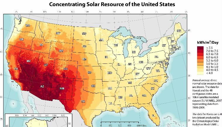
The best CSP is in just a few unpopulated, drought-stricken states (AZ, CA, NM, NV)(NREL 2012):

CSP NREL solar resource 2012

The Seasonal Nature of sunshine (International Energy Agency. 2011. Solar Energy Perspectives)

Seasonal storage for CSP plants would require stone storage. The volume of stone storage for a 100 MW system would be no less than 2 million m3, which is the size of a moderate gravel quarry, or a silo of 250 meter diameter and 67 meter high. This may not be out of proportion, in regions where available space is abundant, as suggested by the comparison with the solar collector field required for a CSP plant producing 100 MW on annual average.

Stones are poor heat conductors, so exchange surfaces should be maximized, for example, with packed beds loosely filled with small particles. One option is then to use gases as HTFs from and to the collector fields, and from and to heat exchangers where steam would be generated. Another option would be to use gas for heat exchanges with the collectors, and have water circulating in pipes in the storage facility, where steam would be generated. This second option would simplify the general plan of the plant, but heat transfers between rocks and pressurized fluids in thick pipes may be problematic.

Annual storage may emerge as a useful option, as generation of electricity by CSP plant in winter is significantly less than in other seasons in the range of latitudes – between 15° and 35° – where suitable areas for CSP generation are found. However, skeptics point out the need for much thicker insulation walls as a critical cost factor.

Square miles needed to produce 25,000 TWh/year with CSP

CSP is more efficient than PV per surface of collectors, but less efficient per land surface, so its 25,000 TWh of yearly production would require a mirror surface of 38,610 square miles (100,000 sq km) and a land surface of about 115,831 square miles (300,000 km2).

Best locations for CSP

Tropical zones thus receive more radiation per surface area on yearly average than the places that are north of the Tropic of Cancer or south of the Tropic of Capricorn. Independent of atmospheric absorption, the amount of available irradiance thus declines, especially in winter, as latitudes increase. The average extraterrestrial irradiance on a horizontal plane depends on the latitude (Figure 2.4).

IEA 2011 figure 2.4 average yearly irradiance by latitude

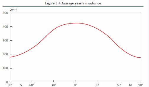
Irradiance varies over the year at diverse latitudes – very much at high latitudes, especially beyond the polar circles, and very little in the tropics (Figure 2.5).  Seasonal variations are greater at higher latitudes:

IEA 2011 figure 2.5 total daily irradiance on a plane horizontal to earth surface

IEA 2011 figure 2.8 yearly profile mean daily solar radiation

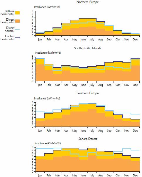
Figure 2.8 The yearly profile of mean daily solar radiation for different locations around the world. The dark area represents direct horizontal irradiance, the light area diffuse horizontal irradiance. Their sum, global horizontal irradiance (GHI) is the black line. The blue line represents direct normal irradiance (DNI). Key point: Temperate and humid equatorial regions have more diffuse than direct solar radiation.

So for solar CSP, the blue line is important and needs to be above 6 for a project to be commercially viable.  The South Pacific Islands have too much moisture (blue line), and northern europe likewise plus not enough irradiance.  Concentrating technologies can be deployed only where DNI largely dominates the solar radiation mix, i.e. in sunny countries where the skies are clear most of the time, over hot and arid or semi-arid regions of the globe. These are the ideal places for concentrating solar power (CSP), concentrating photovoltaics (CPV).  PV can work fine in humid regions, but not CSP or CPV.

Formulations such as “a daily average of 5.5 hours of sunshine over the year” are casually used, however, to mean an average irradiance of 5.5 kWh/m2/d (2 000 kWh/m2/y), i.e. the energy that would have been received had the sun shone on average for 5.5 hours per day with an irradiance of 1,000 W/m2. In this case, one should preferably use “peak sunshine” or “peak sun hours” to avoid any confusion with the concept of sunshine duration.

Ground data measurements for 1-2 years before building a CSP plant

Ground measurements are critically necessary for a reliable assessment of the solar energy possibilities of sites, especially if the technology is CSP or CPV. Satellite data can be used to complement short ground measurement periods of one or two years with a longer term perspective. Ten years is the minimum necessary to have a real perspective on annual variability, and to get a sense of the actual average potential and the possible natural deviations from year to year. Satellite data should be used only when they have been bench-marked by ground measurements.

All parabolic trough plants currently in commercial operation rely on a synthetic oil as heattransfer fluid (HTF) from collector pipes to heat exchangers, where water is preheated, evaporated and then superheated. The superheated steam runs a turbine, which drives a generator to produce electricity. After being cooled and condensed, the water returns to the heat exchangers. Parabolic troughs are the most mature of the CSP technologies and form the bulk of current commercial plants. Investments and operating costs have been dramatically reduced, and performance improved, since the first plants were built in the 1980s. For example, special trucks have been developed to facilitate the regular cleaning of the mirrors, which is necessary to keep performance high, using car-wash technology to save water.

Most first-generation plants have little or no thermal storage and rely on combustible fuel as a firm capacity back-up. CSP plants in Spain derive 12% to 15% of their annual electricity generation from burning natural gas. More than 60% of the Spanish plants already built or under construction, however, have significant thermal storage capacities, based on two-tank molten-salt systems, with a difference of temperatures between the hot tank and the cold one of about 100°C.

Salt mixtures usually solidify below 238°C and are kept above 290°C for better viscosity, however, so work is needed to reduce the pumping and heating expenses required to protect the field against solidifying [my comment: so fossil energy to keep the salts hot subtracts from efficiency]

Energy storage

Worldwide energy storage: The volume of electricity storage necessary to make the electricity available when needed would likely be somewhere between 25 TWh and 150 TWh – i.e. from 10 to 60 hours of storage. If 20 TWh are transferred from one hour to another every day, then the yearly amount of variable renewable electricity shifted daily would be roughly 7,300 TWh. Allowing for 20% losses, one may consider 9,125 TWh in and 7,300 TWh out per year.

Studies examining storage requirements of full renewable electricity generation in the future have arrived at estimates of hundreds of GW for Europe (Heide, 2010), and more than 1,000 GW for the United States (Fthenakis et al., 2009). Scaling-up such numbers to the world as a whole (except for the areas where STE/CSP suffices to provide dispatchable generation) would probably suggest the need for close to 5,000 GW to 6,000 GW storage capacities. Allowing for 3,000 GW gas plants of small capacity factor (i.e. operating only 1 000 hours per year) explains the large difference from the 2,500 GW of storage capacity needs estimated above. However, one must consider the role that large-scale electric transportation could possibly play in dampening variability before considering options for large-scale electricity storage.

V2G possibilities certainly need to be further explored. They do entail costs, however, as battery lifetimes depend on the number, speeds and depths of charges and discharges, although to different extents with different battery technologies. Car owners or battery-leasing companies will not offer V2G free to grid operators, not least because it reduces the lifetime of batteries. Electric batteries are about one order of magnitude more expensive than other options available for large-scale storage, such as pumped-hydro power and compressed air electricity storage.

IEA 2014. Technology Roadmap. Solar Thermal Electricity. International Energy Agency

Global horizontal irradiance (GHI) is a measure of the density of the available solar resource per unit area on a plane horizontal to the earth’s surface. Global normal irradiance (GNI) and direct normal irradiance (DNI) are measured on surfaces “normal” (i.e., perpendicular) to the direct sunbeam. GNI is relevant for two-axis, sun-tracking, “1-sun” (i.e., non-concentrating) PV devices.

DNI is the only relevant metric for devices that use lenses or mirrors to concentrate the sun’s rays on smaller receiving surfaces, whether concentrating photovoltaics (CPV) or CSP generating STE. All places on earth receive 4,380 daylight hours per year — i.e., half the total duration of a year – but different areas receive different yearly average amounts of energy from the sun.

When the sun is lower in the sky, its energy is spread over a larger area and energy is also lost when passing through the atmosphere, because of increased air mass; the solar energy received is therefore lower per unit horizontal surface area.

Inter-tropical areas should thus receive more radiation per land area on a yearly average than places north of the Tropic of Cancer or south of the Tropic of Capricorn.

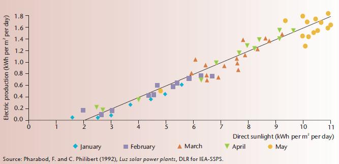
However, atmospheric absorption characteristics affect the amount of this surface radiation significantly. In humid equatorial places, the atmosphere scatters the sun’s rays. DNI is much more affected by clouds and aerosols than global irradiance. The quality of DNI is more important for CSP plants than for concentrated photovoltaics (CPV), because the thermal losses of a CSP plant’s receiver and the parasitic consumption of the electric auxiliaries are essentially constant, regardless of the incoming solar flux. Below a certain level of daily DNI, the net output is null (Figure 2 above).

High DNI is found in hot and dry regions with reliably clear skies and low aerosol optical depths, which are typically in subtropical latitudes from 15° to 40° north or south. Closer to the equator, the atmosphere is usually too cloudy, especially during the rainy season. At higher latitudes, weather patterns also produce frequent cloudy conditions, and the sun’s rays must pass through more atmosphere mass to reach the power plant. DNI is also significantly higher at higher elevations, where absorption and scattering of sunlight due to aerosols can be much lower. Thus, the most favorable areas for CSP resource are in North Africa, southern Africa, the Middle East, north- western India, the south-western United States, northern Mexico, Peru, Chile, the western parts of China and Australia. Other areas that are suitable include the extreme south of Europe and Turkey, other southern US locations, central Asian countries, places in Brazil and Argentina, and some other parts of China.

Areas with sufficient direct irradiance for CSP development are usually arid and many lack water for condenser cooling (Box 1). Dry-cooling technologies for steam turbines are commercially available, so water scarcity is not an insurmountable barrier, but it leads to an efficiency penalty and an additional cost. Wet-dry hybrid cooling can significantly improve performance, with water consumption limited to heat waves.

Almost all existing CSP plants use some fossil fuel as back-up, to remain dispatchable even when the solar resource is low and to guarantee an alternative thermal source that can compensate night thermal losses, prevent freezing and assure a faster start-up in the early morning.

Investment costs for CSP plants have remained high, from USD 4 000/kW to 9 000/kW, depending on the solar resource and the capacity factor, which also depends on the size of the storage system and the size of the solar field, as reflected by the solar multiple.

Costs were expected to decrease as CSP deployment progressed, following a learning rate of 10% (i.e., 10% cost reduction for each cumulative capacity doubling). This decrease has taken a long time to materialize, however, because market opportunities for CSP plants have diminished and the cost of materials has increased, particularly in the most mature parts of the plants, the power block and balance of plant (BOP). Other causes are the dominance of a single technology (trough plants with oil as heat transfer fluid

The few larger plants that have been or are being built elsewhere are either the first of their find in the world, with large development costs and technology risks (e.g., in the United States),

Levelized cost of electricity (LCOE)3 of STE varies widely with the location, technology, design and intended use of plants. The location determines the quantity and quality of the solar resource (Box 1), atmospheric attenuation at ground level, variations in temperature that affect efficiency (e.g., cold at night increases self-consumption, warmth during daylight reduces heat losses but also thermodynamic cycle efficiency) and the availability of cooling water. A plant designed for peak or mid-peak generation with a large turbine for a relatively small solar field will generate electricity at a higher cost than a plant designed for base load generation with a large solar field for a relatively small turbine. LCOE, while providing useful information, does not represent the entire economic balance of a CSP plant, which depends on the value of the generated STE.

Recent CSP plant in the United States secured PPA at USD 135/MWh, but taking investment tax credit into account, the actual remuneration is about USD 190/MWh.  The US DoE’s Sunshot program expects more rapid cost reductions based on current trends, and even aims for LCOE of USD 60/MWh as soon as 2020 [dream on…]

Barriers encountered, overcome or outstanding

Developers have encountered several barriers to establishing CSP plants. These include insufficiently accurate DNI data; inaccurate environmental data; policy uncertainty; difficulties in securing land, water and connections; permitting issues; and expensive financing, leading to difficult financial closure Inaccurate DNI data can lead to significant design errors. Ground-level atmospheric turbidity, dirt, sand storms and other weather characteristics or events may seriously interfere with CSP technologies. Permits for plants have been challenged in courts because of concerns about their effects on wildlife, biodiversity and water use. Some countries prohibit the large-scale use as HTF of synthetic oil or some molten salts, or both.

The most significant barrier is the large up-front investment required. The most mature technology, PT with oil as HTF, with over 200 cumulative years of running, may have limited room for further cost reductions, as the maximum temperature of the HTF limits the possible increase in efficiency and imposes high costs to thermal storage systems. Other technologies offer greater prospects for cost reductions but are less mature and therefore more difficult to obtain finance for. In countries with no or little experience of the technology, financing circles fear risks specific to each country.

In the United States, the loan guarantee program of the DoE has played a key role in overcoming financing difficulties and facilitating technology innovation.

Medium-term outlook

There are no new CSP projects in Spain, as incentives have been cut.

Plants in the approval process or ready to start construction represent 20 MW in France and 115 MW in Italy, while other projects are under development. The Italian environment legislation does not allow for extensive use of oil in trough plants, limiting the technology options to more innovative designs, such as DSG or molten salts as HTF. Projects that would produce several gigawatts are still under consideration or development in the United States, although not all will succeed in obtaining the required permits, PPAs, connections, and financing.

Current average LCOE is high because most existing plants have been built in Spain, which has relatively weak DNI. [my comment: if there is money for energy projects it’s spent regardless of how expensive and foolish – look at all the fracked natural gas by companies deeply in debt, the massive building of solar PV and CSP in Spain, ethanol subsidies, and all kinds of wasteful projects (and research) across the board.  I think this is why there’s no funding for EROI research — nobody wants to know!  Plus foolish projects provide jobs, it’s more important for democrats to provide “green” jobs than whether or not it’s a good idea. And why not, as long as there is oil we can build cities like Las Vegas in the desert that will be abandoned as soon as 2024 or whenever Lake Mead dries up, parking lots, cheap ugly housing projects, and so on]

As deployment intensifies in the southwestern United States and spreads to North Africa, South Africa, Chile, Australia and the Middle East, better resources will be used, improving performance.

Table 4: Projections of LCOE for new-built CSP plants with storage in the hi-Ren Scenario

The possible role of small-scale CSP devices – from 100 kW to a few MW – off-grid or serving in mini-grids, has not been included in the ETP model. There is too little industrial experience of such systems to make informed cost assumptions, whether the systems are based on PT, LFR, parabolic dishes, Scheffler dishes or small towers, using organic Rankin cycle turbines, micro gas-turbines or various reciprocating engines. If they allow thermal storage4 or fuel backup, small-scale CSP systems have to compete against PV with battery storage or fuel backup. They may find a role, although the fact that CSP technology seems to benefit more than PV from economies of scale suggests that smallscale CSP systems may face a greater competitive challenge than large-scale ones. Finding local skills for maintenance may also be challenging in remote, off-grid areas.

Storage is a particular challenge in CSP plants that use DSG. Because water evaporation is isothermal, unlike sensible heat addition or removal in the salt, a round-trip storage cycle would result in severe steam temperature and pressure drops, thereby destroying the efficiency of the thermodynamic cycle in discharge mode. Storing latent heat of saturated steam in pressurised vessels is expensive and provides no scale effect on cost. One option would use three-stage storage devices that preheat the water, evaporate the water and superheat the steam. Stages 1 and 3 would be sensible heat storage, in which the temperature of the storage medium changes. Stage 2 would best be latent heat storage, in which the state of the storage medium changes, using some phase change material. Another option could be to use liquid phase-change materials. The growing relevance of thermal storage in the context of intense competition from cheap PV favors using molten salts as both the heat transfer fluid and the storage medium (termed “direct storage”). If DSG spares heat exchangers for steam generation, the use of molten salts as HTF spares heat exchangers for storage. Salts are less costly than oil. Using salts allows raising the temperature and pressure of the steam, from 380°C to 530-550°C and from 10 to 12-15 megapascals (MPa) in comparison with oil as HTF, increasing the efficiency of the power block from 39% to 44-45% (Lenzen, 2014). Thanks to higher temperature differences between hot and cold salts (currently used salt mixtures usually solidify below 238°C), plants using molten salts as HTF need three times less salts than trough plants using oil as HTF, for the same storage capacity. This lowers the storage system costs, which represent about 12% of the overall plant cost for seven-hour storage of a trough plant. Also, the “return efficiency” of thermal storage, at about 93% with indirect storage (in which heat exchangers reduce the working temperature), is increased to 98% with direct storage. Finally, another advantage of molten salts as HTF over steam is that heat transfer can be carried out at low pressure with thin-wall solar receivers, which are cheaper and more effective. Overall, the substitution of molten salts for oil in CSP would allow for 30% LCOE reduction, according to Schott, the lead manufacturer of solar receiver tubes (Lenzen, 2014). Several companies are developing the use of molten salts as HTF in linear systems, and have built or are building experimental or demonstration devices. One challenge is to reduce the expense required to keep the salts warm enough (usually above 290°C) for better viscosity in long tubes at all times and protect the field against freezing.

Apart from the fundamental choice between DSG and molten salts for HTF, towers currently also offer a great diversity of designs – and present various trade-offs. The first relates to the size (and number) of heliostats that reflect the sunlight onto the receivers atop the tower. Heliostats vary greatly in size, from about 1 m2 to 160 m2. The small ones can be flat and offer little surface to winds. The larger ones need several mirrors that are curved to send a focused image of the sun to the central receiver, and need strong support structures and motors to resist winds. For similar collected energy ranges, however, small heliostats need to be grouped by the thousand, multiplying the number of motors and connections. Manufacturers and experts still have divided views about the optimum size. Heliostats need to be distanced from one another to reduce losses arising when a heliostat intercepts part of the flux received (“shading”) or reflected (“blocking”) by another. While linear systems require flat land areas, central receiver systems may accommodate some slope, or even benefit from it as it could reduce blocking and shadowing, and allow increasing heliostat density. Algorithmic field optimization may help reduce environmental impacts and required ground leveling work while maximizing output (Gilon, 2014).

In low latitudes heliostat fields tend to be circular and surround the central receiver, while in higher latitudes they tend to be more concentrated to the polar side of the tower. Larger fields tend to be more circular to limit the maximum receiver heliostat distance and minimise atmospheric attenuation.

Proper aiming strategy must be ensured by the heliostat field’s control system in order to optimise the solar flux map on the receiver, thereby allowing the highest solar input while avoiding any local overheating of the receiver tubes. This is more difficult with DSG receivers. The heat flux on the different types of solar panel of a DSG receiver differs significantly: superheater panels (poorly cooled by superheated steam) receive a much lower flux than evaporator and preheater panels. Another important design choice relates to the number of towers for one turbine. Heliostats that are in the last rows far from the tower need to be very precisely pointed towards it, and lose efficiency as the light must make a long trip near ground level. They also have greater geometrical (“cosine”) optical losses.

At over 1 million m2, the solar field associated with the 110 MW tower built by SolarReserve with 10-hour storage at Crescent Dunes, (Nevada, United States) is perhaps close to the maximum efficient size.

The additional costs of building several towers may be made up for by the greater optical and thermal efficiencies of multitower design (Wieghardt et al., 2014). However, the optimal field size and number of towers may depend on the atmospheric turbidity of the site considered, which varies greatly among areas suitable for CSP plants. The Californian company eSolar proposes 100 MW molten salt power plants based on 14 solar fields and 14 receivers on top of monopole towers (similar to current large wind turbine masts) for one central dry-cooled power block with 13-hour thermal storage and 75% capacity factor (Tyner, 2013).

As the share of variable energy increases, base load plants, even if technically flexible (which all are not) will become less economically efficient as their utilization rate diminishes. At the same time, more peaking and mid-merit plants become necessary. Below a certain load factor – about 2,000 full load hours – open-cycle gas turbines become a better economic choice than combined-cycle plants, but they are less energy-efficient as they generate large amounts of waste heat.

Open-cycle gas turbines could be integrated with a CSP plant with storage, however, of which the steam turbine is not being used with a very high capacity factor. When the sun does not shine, the otherwise wasted heat could be collected to a large extent in the hot tank of a two-tank molten-salt system. This energy could afterwards be directed to the steam turbine to deliver electricity whenever requested. If more power is needed when the sun shines sufficiently to run the steam turbine by itself, the heat from the gas turbine could be directed to the thermal storage. In both cases, a large part of the waste heat will be used. This concept differs from the existing ISCC in which solar only provides a complement, as the presence of thermal storage allows for a complete reversal of the proportion of solar and gas, which remains a backup, though a more efficient one (Crespo, 2014). The Hysol project, funded by the European Union’s Seventh Program for research, technological development and demonstration, aims to demonstrate the viability of the concept. Similarly, in areas with both high wind penetration and CSP plants, some thermal storage, which is equipped with electric heaters for security reasons, could be used in winter to reduce curtailment from excess wind power.

Molten salts decompose at higher temperatures, while corrosion limits the temperatures of steam turbines. Higher temperatures and efficiencies could rest on the use of fluoride liquid salts as HTFs up to temperatures of 700°C to 850°C,

There are a number of potential pathways to solar fuels. The straightforward thermolysis of water is the most difficult, as it requires temperatures above 2 200°C and may produce an explosive mixture of hydrogen and oxygen. The division of the single-step water-splitting reaction into a number of sub- reactions opens up the field of so called thermochemical cycles for H2 production. The necessary reaction temperature can be decreased even below 1 000°C, resulting in intermediate solid products like metals (e.g., aluminium, magnesium, or zinc), metal oxides, metal halides or sulphur oxides. The different reaction steps can be separated in time and place, offering possibilities for long-term storage of the solids and their use in transportation. These thermochemical cycles are also able to split CO2 into CO and oxygen. If mixtures of water and CO2 are used, even synthesis gas (mainly H2 and CO) can be produced, which can be further processed to synfuels, for example by the Fischer-Tropsch process.

Concentrated solar radiation can also be used to upgrade carbonaceous materials. The most developed process is the steam reforming of methane to produce synthesis gas. Sources are either natural gas or biogas. Methane can also be cracked into hydrogen and carbon, thus producing a gaseous and a solid product. However, the required process temperature is extremely high and a homogeneous carbon product is unlikely to be produced because of the intermittent solar radiation conditions. Additionally, there is a discrepancy between the huge demand for hydrogen and the low demand for high-value carbon, such as carbon black or advanced carbon nano-tubes.

Hydrogen produced in concentrating solar chemical plants could be blended with natural gas and thus used in today’s energy system. Town gas, which prevailed before natural gas spread out, included hydrogen up to 60% in volume or about 20% in energy content. This blend could be used for various purposes in industry, households and transportation, reducing emissions of CO2 and nitrous oxides. Gas turbines in integrated gasification combined cycle (IGCC) power plants can burn a mix of gases with 90% hydrogen in volume. Many existing pipelines could, with some adaptation, transport such a blend from sunny places to large consumption centres (e.g. from North Africa to Europe).

Solar-produced hydrogen could also find niche markets today in replacing hydrogen production from steam-reforming of natural gas in its current uses, such as manufacturing fertilizers and removing sulfur from petroleum products. Regenerating hydrogen with heat from concentrated sunlight to decompose hydrogen sulphide into hydrogen and sulfur could save significant amounts of still gas in refineries for other purposes. Coal could be used together with methane gas as feedstock, and deliver dimethyl ether (DME), after solar-assisted steam reforming of natural gas, coal gasification under oxygen, and two-step water splitting. DME could be used as a liquid fuel, and its combustion would entail similar CO2 emissions to those from burning conventional petroleum products, but significantly less than the life-cycle emissions of other coal-to-liquid fuels.

Besides solar fuels, CSP technology could find a great variety of uses in providing high temperature process heat or steam, such as for enhanced oil recovery, and mining applications (where CSP is already in use), smelting of aluminium and other metals, and in industries such as food and beverages, textiles and pharmaceuticals. Various forms of cogeneration with STE can also be considered. For example, sugar plants require high temperature steam in spring, when the solar resource is maximal but electricity demand minimal. Solar fields providing steam for sugar plants could run a turbine and generate STE for the rest of the year.

STE is not broadly competitive today, and will not become so until it benefits from strong and stable frameworks, and appropriate support to minimise investors’ risks and reduce capital costs.

As with any large industrial projects, STE projects require several permissions, often delivered by many different government jurisdictions at various geographical levels, as well as many branches or agencies of each – local, regional, state, federal or national. Each may protect different interests, all of them legitimate.

Future values of PV and STE in California Researchers at the National Laboratory of Renewable Energy (NREL) in the United States have studied the future total values (operational value plus capacity value) of STE with storage and PV plants in California in two scenarios: one with 33% renewables in the mix (the renewable portfolio standard by end 2020), including about 11% PV, another with 40% renewables (under consideration by California’s governor), including about 14% PV. In both cases there is over 1 GW of electricity storage available on the grid. The main results indicate that at 33% renewable penetration, the bulk of the gap in favour of STE comes from its greater capacity value, which avoids the costs of building additional thermal generators to meet demand (Table 5). At 40% renewable penetration, the value of STE increases slightly, but the value of PV drops significantly, mostly reflecting the drop of its own capacity value (Jorgenson et al., 2014). For investment decisions and planning, system values are as much important as LCOE. Table 6: Total value in two scenarios of renewables penetration in California Value component 33% renewables 40% renewables STE with storage PV Value value (USD/MWh) (USD/MWh) STE with

The built-in storage capability of CSP is cheaper and more effective (with over 95% return efficiency, versus about 80% for most competing technologies) than battery storage and pumped-hydropower storage. Thermal storage allows separating the collection of the heat (during the day) and the generation of electricity (at will). This capability has immediate value in countries having significant increase in power demand when the sun sets, in part driven by lighting requirements. In many such countries, the electricity mix, which during daytime is often dominated by coal, becomes dominated by peaking technologies, often based on natural gas or oil products.

The greatest possible expansion of PV, which implies its dominance over all other sources during a significant part of the day, creates difficult technical and economic challenges to low-carbon base-load technologies such as nuclear power and fossil fuel with CCS. Natural gas is more suited to daily “stop-and-go” with rapid ramps up and down, and is more economical for mid-merit operations (between about 2,000 and 4,000 full-load hours).

changes in the rules applicable to investments already being made or in process can have long-lasting deterrent effects on investments if they significantly modify the prospects for economic returns. This is precisely what has happened over the last few years in Spain, where a series of measures aimed at reducing the return on investment on existing CSP plants. The high risk of losing investors’ confidence may have been deemed acceptable, as these measures followed the decision to stop CSP deployment. However it may have detrimental effects for future investments in CSP plants; for other investments in the energy sector; for other investments in any other sector that requires government involvement; and for investments in other countries

Financing CSP plants, like most renewable energy plants, are very capital-intensive, requiring large upfront expenditures. Financing is thus difficult, especially in new, immature markets, and for new, emerging sub-technologies. In the United States, some private investors have large amounts of money available and might be willing to invest in clean energy for a variety of reasons; but even in this context the risks may have appeared too high for large, innovative CSP projects – costing around USD 1 billion – to materialize, without the loan guarantee program of the US DoE. This program has been essential to the renaissance of CSP in the United States, in allowing projects to access debt at very low cost from a US government bank and facilitating financial closure at acceptable WACC of large projects.

In other countries, such as India, Morocco and South Africa, public low-cost lending has been essential for jump-starting the deployment of CSP. In India and South Africa, private banks would have not provided capital for the very long maturity involved. In Morocco, the presence of a government agency as equity partner significantly reduced the perception of policy risks among other partners. In Morocco and South Africa, international finance institutions provided concessional grants that reduced the overall costs of large CSP projects.

Subsidizing renewable energy projects through long-term and/or low-cost debt-related policies could reduce the total subsidies compared with per-kWh support. However, this transfers the burden of high capital-intensivity to governments, which may not have enough money at hand, and this carries a risk of slowing deployment. Interest subsidies and/or accelerated depreciation have much higher one-year budget efficiency.

Research is under way to test and evaluate methods of measuring DNI accurately using lower-cost instrumentation, and for producing long-term, high-quality DNI data sets by merging long-term, satellite-derived data of moderate accuracy with high-quality, highly accurate ground-based measurements that may only cover a year or less. This research also includes important studies on sunshape and circumsolar radiation, and how these factor into both DNI measurements and STE system performance. In addition, satellite-based methods for estimating DNI are constantly improving and represent a reliable and viable way of choosing the best sites for STE plants. Furthermore, the ability to accurately forecast DNI levels – from a few hours ahead to a few days ahead – is constantly improving, and will be an important tool for utilities operating STE systems.

Abbreviations: ARRA American recovery and reinvestment Act CCS carbon capture and storage CO2 carbon dioxide CPI Climate Policy Initiative CSF concentrated solar fuels CSP concentrating solar power CPV concentrating photovoltaic CRS central receiver system CTF Clean Technology Fund DC direct current DII Desertec Industry Initiative DLR Forschungszentrum der Bundesrepublik Deutschland für Luft- und Raumfahrt (German Aerospace Centre) DME Dimethyl ether DNI direct normal irradiance DSG direct steam generation EDF Électricité de France EIB European Investment Bank EPC engineering, procurement and construction ETP: Energy Technology Perspectives EU European Union EUR euro FiT feed-in tariff FiP feed-in premium G8 Group of Eight GHG greenhouse gas(es) GHI global horizontal irradiance GNI global normal irradiance Gt gigatonnes GW gigawatt (1 million kW)  GWh gigawatt hour (1 million kWh) Hi-Ren high renewables (Scenario) HTF heat transfer fluid HVDC high- voltage direct current IA implementing agreement IEA International Energy Agency IFI international financial institution IGCC integrated gasification combined cycle IRENA International Renewable Energy Agency ISCC Integrated Solar Combined-Cycle (plant) JRC Joint Research Centre kW kilowatt kWh kilowatt hour LCOE levelized cost of electricity LFR linear Fresnel reflectors MW megawatt (1 thousand kW) MWe megawatt electrical MWh megawatt hour (1 thousand kWh) MWth megawatt thermal NGO non-governmental organisation NREAP national renewable energy action plan NREL National Renewable Energy Laboratory (United States) OECD Organization for Economic Co-operation and Development O&M operation and maintenance PPA power purchase agreement PT parabolic trough  TWh terawatthour (1 billion KWh)

IEA (2014a), Technology Roadmap: Solar Photovoltaic Energy, 2014 Edition, OECD/IEA, Paris. IEA (2014b), Energy Technology Perspectives 2014, OECD/IEA, Paris. IEA (2014c), Technology Roadmap: Energy Storage, OECD/IEA, Paris. IEA (2014d), Medium-Term Renewable Energy Market Report, OECD/IEA, Paris. IEA (2014e), The Power of Transformation: Wind, Sun and the Economics of Flexible Power Systems, OECD/ IEA, Paris. IEA (2011), Solar Energy Perspectives, Renewable Energy Technologies, OECD/IEA, Paris. IEA (2010), TechnologyRoadmap: Concentrating Solar Power, OECD/IEA, Paris.

Jorgenson, J., P. Denholm and M. Mehos (2014), Estimating the Value of Utility-Scale Solar Technologies in California under a 40% Renewable Portfolio Standard, NREL/TP-6A20-61695, May.

RED electrica de España (REE) (2014), The Spanish Electricity System – Preliminary Report 2013, RED, Madrid, Spain, http://www.ree.es/sites/default/files/downloadable/preliminary_report_2013.pdf.

REFERENCES

Deign, J. 2020. America’s Concentrated Solar Power Companies Have All but Disappeared. greentechmedia.com

DOE/NETL. August 28, 2012. Role of Alternative Energy Sources: Solar Thermal Technology Assessment. Department of Energy, National Energy Technology Laboratory.

Martin, C., et al. 2020. A $1 Billion Solar Plant Was Obsolete Before It Ever Went Online. SolarReserve’s Crescent Dunes received backing from Citigroup and the Obama Energy Department but couldn’t keep pace with technological advances. Bloomberg.

NREL. 2011a. Solar Radiation Data Manual for Flat Plate and Concentrating Collectors. National Renewable Energy Laboratory.

NREL. 2011b. U.S. Solar Radiation Resource Maps: Atlas for the Solar Radiation Data Manual for Flat Plate and Concentrating Collectors. National Renewable Energy Laboratory.

Maps: http://www.nrel.gov/gis/solar.html

NREL. 2012. Concentrating solar resource of the united states. National Renewable Energy Laboratory.

Posted in Concentrated Solar Power, CSP with thermal energy storage, Grid instability, Seasonal Variation | Tagged , , , , , | 1 Comment

Oil consumption of containerships

This image has an empty alt attribute; its file name is container-ship.jpg
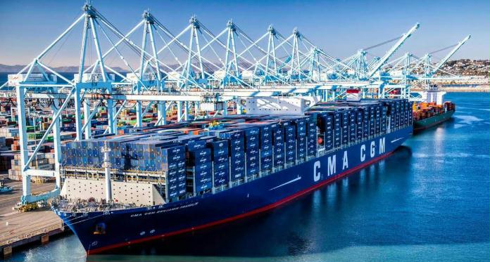
Preface.  Since 90% of international goods move by ships, I was curious about how much fuel they burned.  It’s a lot: The very large container ship CMA CGM Benjamin Franklin above, which can carry 18,000 20-foot containers, carries approximately 4.5 million gallons of fuel oil, which takes up 16,000 cubic meters (FW 2020).  As much fuel as 300,000 15-gallon tank cars.

But these ships can carry 200,000 tons of goods, so they end up being more energy efficient than 300,000 cars (Stopford 2010, UNCTAD 2012).

Pound for pound and mile for mile, today’s ships are the most energy-efficient way to move freight. Table 1 shows the energy efficiency of different modes of transport by kilojoules of energy used to carry one ton of cargo a kilometer (KJ/tkm). As you can see, water and rail are literally tons and tons—orders of magnitude—more energy efficient than trucks and air transportation.

Table 1 Energy efficiency of transportation in kilojoules/ton/kilometer (Smil 2013), Ashby 2015)

(A) ……………Transportation mode
50……………. Oil tankers and bulk cargo ships
100–150….. Smaller cargo ships
250–600….. Trains
360………….. Barge
2000–4000 Trucks
30,000…….. Air freight
55,000…….. Helicopter

(A) Kilojoules of energy used to carry one ton of cargo one kilometer Transportation mode

Alice Friedemann www.energyskeptic.com  author of “When Trucks Stop Running: Energy and the Future of Transportation”, 2015, Springer, Barriers to Making Algal Biofuels, and “Crunch! Whole Grain Artisan Chips and Crackers”. Podcasts: Collapse Chronicles, Derrick Jensen, Practical Prepping, KunstlerCast 253, KunstlerCast278, Peak Prosperity , XX2 report

***

Further details

Fuel consumption by a container ship is mostly a function of ship size and cruising speed, which follows an exponential function above 14 knots. So an 8,000 TEU container ship consumes 225 tons of bunker fuel per day at 24 knots, but at 21 knots  consumption drops to 150 tons per day, a 33% decline. While shipping lines would prefer consuming the least amount of fuel by adopting lower speeds, this advantage must be mitigated with longer shipping times as well as assigning more ships on a pendulum service to maintain the same port call frequency. The main ship speed classes are (Notteboom 2009):

  • Normal (20-25 knots; 37.0 – 46.3 km/hr). Represents the optimal cruising speed a containership and its engine have been designed to travel at. It also reflects the hydrodynamic limits of the hull to perform within acceptable fuel consumption levels. Most containerships are designed to travel at speeds around 24 knots.
  • Slow steaming (18-20 knots; 33.3 – 37.0 km/hr). Running ship engines below capacity to save fuel consumption, but at the expense a additional travel time, particularly over long distances (compounding effect). This is likely to become the dominant operational speed as more than 50% of the global container shipping capacity was operating under such conditions as of 2011.
  • Extra slow steaming (15-18 knots; 27.8 – 33.3 km/hr). Also known as super slow steaming or economical speed. A substantial decline in speed for the purpose of achieving a minimal level of fuel consumption while still maintaining a commercial service. Can be applied on specific short distance routes.
  • Minimal cost (12-15 knots; 22.2 – 27.8 km/hr). The lowest speed technically possible, since lower speeds do not lead to any significant additional fuel economy. The level of service is however commercially unacceptable, so it is unlikely that maritime shipping companies would adopt such speeds.

In an environment of higher fossil fuel prices, maritime shipping companies are opting for slow steaming for cost cutting purposes.   The ongoing practice of slow steaming is likely to have an impact on supply chain management, maritime routes and the use of transshipment hubs.

REFERENCES

Ashby, M.F. 2015. Materials and sustainable development, table A.14. Oxford: Butterworth-Heinemann.

FW. 2020. How many gallons of fuel does a container ship carry? freightwaves.com

Smil, V. 2013. Prime movers of globalization. The history and impact of diesel engines and gas turbines. Cambridge: The MIT press.

Stopford, M. 2010. How shipping has changed the world and the social impact of shipping. Global Maritime Environmental Congress.

Notteboom, T., et al. 2009. Fuel surcharge practices of container shipping lines: Is it about cost recovery or revenue making?. Proceedings of the 2009 International Association of Maritime Economists (IAME) Conference, June, Copenhagen, Denmark.

UNCTAD. 2012. Review of maritime transport. United Nations.

Posted in Electrification, Ships and Barges | Tagged , | 2 Comments

Life before Cars: When Pedestrians Ruled the Streets

This image has an empty alt attribute; its file name is horses-before-cars.jpg

Preface.  The past is future after fossil fuels, but minus the horses for a while, since before cars they required about a sixth of U.S. farmland for their feed.  My grandfather, Francis J. Pettijohn, used to fondly reminisce about how quiet it used to be before combustion engines in his small town in Minnesota, though in cities that wasn’t the case, the clatter of wagon wheels on cobblestones was excruciatingly loud.

Alice Friedemann www.energyskeptic.com  author of “When Trucks Stop Running: Energy and the Future of Transportation”, 2015, Springer, Barriers to Making Algal Biofuels, and “Crunch! Whole Grain Artisan Chips and Crackers”. Podcasts: Collapse Chronicles, Derrick Jensen, Practical Prepping, KunstlerCast 253, KunstlerCast278, Peak Prosperity , XX2 report

***

Clive Thompson. December 2014. When Pedestrians Ruled the Streets  Smithsonian Magazine.

When you visit any city in America today, it’s a sea of cars, with pedestrians dodging between the speeding autos. It’s almost hard to imagine now, but in the late 1890s, the situation was completely reversed. Pedestrians dominated the roads, and cars were the rare, tentative interlopers. Horse-drawn carriages and streetcars existed, but they were comparatively slow.

So pedestrians ruled. “The streets were absolutely black with people,” as one observer described the view in the nation’s capital. People strolled to and fro down the center of the avenue, pausing to buy snacks from vendors. They’d chat with friends or even “manicure your nails,” as one chamber of commerce wryly noted. And when they stepped off a sidewalk, they did it anywhere they pleased.

“They’d stride right into the street, casting little more than a glance around them…anywhere and at any angle,” as Peter D. Norton, a historian and author of Fighting Traffic: The Dawn of the Motor Age in the American City, tells me. “Boys of 10, 12 or 14 would be selling newspapers, delivering telegrams and running errands.” For children, streets were playgrounds.

At the turn of the century, motor vehicles were handmade, expensive toys of the rich, and widely regarded as rare and dangerous. When the first electric car emerged in Britain in the 19th century, the speed limit was set at four miles an hour so a man could run ahead with a flag, warning citizens of the oncoming menace, notes Tom Vanderbilt, author of Traffic: Why We Drive the Way We Do (And What It Says About Us).

Things changed dramatically in 1908 when Henry Ford released the first Model T. Suddenly a car was affordable, and a fast one, too: The Model T could zoom up to 45 miles an hour. Middle-class families scooped them up, mostly in cities, and as they began to race through the streets, they ran headlong into pedestrians—with lethal results. By 1925, auto accidents accounted for two-thirds of the entire death toll in cities with populations over 25,000.

An outcry arose, aimed squarely at drivers. The public regarded them as murderers. Walking in the streets? That was normal. Driving? Now that was aberrant—a crazy new form of selfish behavior.

“Nation Roused Against Motor Killings” read the headline of a typical New York Times story, decrying “the homicidal orgy of the motor car.” The editorial went on to quote a New York City traffic court magistrate, Bruce Cobb, who exhorted, “The slaughter cannot go on. The mangling and crushing cannot continue.” Editorial cartoons routinely showed a car piloted by the grim reaper, mowing down innocents.

When Milwaukee held a “safety week” poster competition, citizens sent in lurid designs of car accident victims. The winner was a drawing of a horrified woman holding the bloody corpse of her child. Children killed while playing in the streets were particularly mourned. They constituted one-third of all traffic deaths in 1925; half of them were killed on their home blocks. During New York’s 1922 “safety week” event, 10,000 children marched in the streets, 1,054 of them in a separate group symbolizing the number killed in accidents the previous year.

Drivers wrote their own letters to newspapers, pleading to be understood. “We are not a bunch of murderers and cutthroats,” one said. Yet they were indeed at the center of a fight that, clearly, could only have one winner. To whom should the streets belong?

***

By the early 1920s, anti-car sentiment was so high that carmakers and driver associations—who called themselves “motordom”—feared they would permanently lose the public.

You could see the damage in car sales, which slumped by 12 percent between 1923 and 1924, after years of steady increase. Worse, anti-car legislation loomed: Citizens and politicians were agitating for “speed governors” to limit how fast cars could go. “Gear them down to fifteen or twenty miles per hour,” as one letter-writer urged. Charles Hayes, president of the Chicago Motor Club, fretted that cities would impose “unbearable restrictions” on cars.

Hayes and his car-company colleagues decided to fight back. It was time to target not the behavior of cars—but the behavior of pedestrians. Motordom would have to persuade city people that, as Hayes argued, “the streets are made for vehicles to run upon”—and not for people to walk. If you got run over, it was your fault, not that of the motorist. Motordom began to mount a clever and witty public-relations campaign.

Their most brilliant stratagem: To popularize the term “jaywalker.” The term derived from “jay,” a derisive term for a country bumpkin. In the early 1920s, “jaywalker” wasn’t very well known. So pro-car forces actively promoted it, producing cards for Boy Scouts to hand out warning pedestrians to cross only at street corners. At a New York safety event, a man dressed like a hayseed was jokingly rear-ended over and over again by a Model T. In the 1922 Detroit safety week parade, the Packard Motor Car Company produced a huge tombstone float—except, as Norton notes, it now blamed the jaywalker, not the driver: “Erected to the Memory of Mr. J. Walker: He Stepped from the Curb Without Looking.”

The use of “jaywalker” was a brilliant psychological ploy. What’s the best way to convince urbanites not to wander in the streets? Make the behavior seem unsophisticated—something you’d expect from hicks fresh off the turnip truck. Car companies used the self-regarding snobbery of city-dwellers against themselves. And the campaign worked. Only a few years later, in 1924, “jaywalker” was so well-known it appeared in a dictionary: “One who crosses a street without observing the traffic regulations for pedestrians.”

Meanwhile, newspapers were shifting allegiance to the automakers—in part, Norton and Vanderbilt argue, because they were profiting heavily from car ads. So they too began blaming pedestrians for causing accidents.

“It is impossible for all classes of modern traffic to occupy the same right of way at the same time in safety,” as the Providence Sunday Journal noted in a 1921 article called “The Jay Walker Problem,” reprinted from the pro-car Motor magazine.

In retrospect, you could have predicted that pedestrians were doomed. They were politically outmatched. “There was a road lobby of asphalt users, but there was no lobby of pedestrians,” Vanderbilt says. And cars were a genuinely useful technology. As pedestrians, Americans may have feared their dangers—but as drivers, they loved the mobility.

By the early ’30s, the war was over. Ever after, “the street would be monopolized by motor vehicles,” Norton tells me. “Most of the children would be gone; those who were still there would be on the sidewalks.” By the 1960s, cars had become so dominant that when civil engineers made the first computer models to study how traffic flowed, they didn’t even bother to include pedestrians.

***

The triumph of the automobile changed the shape of America, as environmentalists ruefully point out. Cars allowed the suburbs to explode, and big suburbs allowed for energy-hungry monster homes. Even in mid-century, critics could see this coming too. “When the American people, through their Congress, voted for a 26-billion-dollar highway program, the most charitable thing to assume is that they hadn’t the faintest notion of what they were doing,” Lewis Mumford wrote sadly in 1958.

Posted in Automobiles, Transportation What To Do | Tagged | 1 Comment

15 Nations that Collapsed because of Drought: will we be the 16th?

Preface.  Another repercussion of drought may be the Muslim religion as Fleitmann (2022) proposes below.

This post began with 10 civilizations that collapsed due to drought (below), and I’ve added 5 more. Will the American South West be #16? Lynn Ingram, a professor at U.C. Berkeley discusses this possibility in her  book: The West without Water: What Past Floods, Droughts, and Other Climatic Clues Tell Us about TomorrowSince 2000, California and the South West have had the worst drought in 1,200 years.  Since California’s aquifer and the Ogallala under 10 states produce half of America’s food, the rest of the nation won’t escape…

Alice Friedemann  www.energyskeptic.com  Author of Life After Fossil Fuels: A Reality Check on Alternative Energy; When Trucks Stop Running: Energy and the Future of Transportation”, Barriers to Making Algal Biofuels, & “Crunch! Whole Grain Artisan Chips and Crackers”.  Women in ecology  Podcasts: WGBH, Jore, Planet: Critical, Crazy Town, Collapse Chronicles, Derrick Jensen, Practical Prepping, Kunstler 253 &278, Peak Prosperity,  Index of best energyskeptic posts

***

Fleitmann D et al (2022) Droughts and societal change: The environmental context for the emergence of Islam in late Antique Arabia. Science 376: 1317-1321

In Arabia, the first half of the sixth century CE was marked by the demise of Himyar, the dominant power in Arabia until 525 CE. Important social and political changes followed, which promoted the disintegration of the major Arabian polities. Using hydroclimate and stalagmite records from around Southern Arabia, we clearly see unprecedented droughts during the sixth century CE, with the worst of it from ~500 to 530 CE. We suggest that such droughts undermined the resilience of Himyar and thereby contributed to the societal changes from which Islam emerged.

Scroxton J (2020) Circum-Indian ocean hydroclimate at the mid to late Holocene transition: The Double Drought hypothesis and consequences for the Harappan. Climate Past discussions.

The Harappan arose in the Indus valley near Afghanistan and India about 5200 years ago, peaking around 2600 BC. Their written script remains undeciphered, but archeology has revealed skilled metallurgy, intricate sewer systems, reservoirs, public baths and urban planning long before the Roman Empire. But by 1300 BC it collapsed. Scroxton found a sudden drought starting around 2240 BC affecting winter rain fall, and many fled to present-day Indian Gujarat, while others coped by switching to millet and grains that favored summer rain. Then 300 years later, just as the winter rains began to recover, a tropical drought came, reducing the summer rains for several centuries, greatly reducing the population.

Sinha A et al (2019) Role of climate in the rise and fall of the Neo-Assyrian Empire. Science Advances.

New research suggests it was drought that led to the collapse of the Assyrian Empire (whose heartland was based in today’s northern Iraq)—one of the most powerful civilizations in the ancient world.  Neo-Assyria was the first super power in the history of the world. The Neo-Assyrian empire (912-609 BC) was the third and final phase of Assyrian civilization. It was by far the largest empire in the region up to that time, controlling much of the territory from the Persian Gulf to Cyprus. The Assyrians were basically like the Empire in Star Wars, they are the all-devouring machine.

They also had incredible skill as hydro-engineers. The Assyrians were largely responsible for the way that the Tigris River Basin drainage now works, they completely remade the natural water flows of that landscape using aqueducts and other hydraulic infrastructure. Some of these features are still functioning today.

Today Iraq is water challenged, with a low level per capita of fresh water, and until a deluge in the winter of 2019, very little rain since 1988.

Masters J (2016) Ten Civilizations or Nations That Collapsed From Drought.  wunderground

Drought is the great enemy of human civilization. Drought deprives us of the two things necessary to sustain life–food and water. When the rains stop and the soil dries up, cities die and civilizations collapse, as people abandon lands no longer able to supply them with the food and water they need to live. While the fall of a great empire is usually due to a complex set of causes, drought has often been identified as the primary culprit or a significant contributing factor in a surprising number of such collapses. Drought experts Justin Sheffield and Eric Wood of Princeton, in their 2011 book, Drought, identify more than ten civilizations, cultures and nations that probably collapsed, in part, because of drought. As we mark World Water Day on March 22, we should not grow overconfident that our current global civilization is immune from our old nemesis–particularly in light of the fact that a hotter climate due to global warming will make droughts more intense and impacts more severe. So, presented here is a “top ten” list of drought’s great power over some of the mightiest civilizations in world history–presented chronologically.

Collapse #1. The Akkadian Empire in Syria, 2334 BC – 2193 BC. In Mesopotamia 4200 years ago, the great Akkadian Empire united all the indigenous Akkadian-speaking Semites and the Sumerian speakers, and controlled Mesopotamia, the Levant, and parts of Iran, sending military expeditions as far south as present-day Oman. In a 2000 article published in Geology, “Climate change and the collapse of the Akkadian empire: Evidence from the deep sea”, a team of researchers led by Heidi Cullen studied deposits of continental dust blown into the Gulf of Oman in the late 1990s. They discovered a large increase in dust 4200 years ago that likely coincided with a 100-year drought that brought a 30% decline in precipitation to Syria. The drought, called the 4.2 kiloyear event, is thought to have been caused by cooler sea surface temperatures in the North Atlantic. The 4.2 kiloyear event has also been linked to the collapse of the Old Kingdom in Egypt (see below). The paper concluded, “Geochemical correlation of volcanic ash shards between the archeological site and marine sediment record establishes a direct temporal link between Mesopotamian aridification and social collapse, implicating a sudden shift to more arid conditions as a key factor contributing to the collapse of the Akkadian empire.”

Collapse #2. The Old Kingdom of ancient Egypt, 4200 years ago. The same drought that brought down the Akkadian empire in Syria severely shrank the normal floods on the Nile River in ancient Egypt. Without regular floods to fertilize the fields, poor harvests led to reduced tax income and insufficient funds to finance the pharaoh’s government, hastening the collapse of Egypt’s pyramid-building Old Kingdom. An inscription on the tomb of Ankhtifi during the collapse describes the pitiful state of the country when famine stalked the land: “the whole country has become like locusts going in search of food…”

Collapse #3. The Late Bronze Age (LBA) civilization in the Eastern Mediterranean. About 3200 years ago, the Eastern Mediterranean hosted some of the world’s most advanced civilizations. The Mycenaean culture was flourishing in Greece and Crete. The chariot-riding Hittites had carved out a vast empire encompassing a large part of Asa Minor and the Middle East. In Egypt, the New Kingdom was at its height. However, around 1200 BC, these Eastern Mediterranean civilizations declined or collapsed. According to a 2013 study in PLOS, studying grains of fossilized pollen shows that this collapse coincided with the onset of a 300-year drought event. This climate shift caused crop failures and famine, which “precipitated or hastened socio-economic crises and forced regional human migrations at the end of the LBA in the Eastern Mediterranean and southwest Asia.”

Collapse #4. The Maya civilization of 250-900 AD in Mexico. Severe drought killed millions of Maya people due to famine and lack of water, and initiated a cascade of internal collapses that destroyed their civilization at the peak of their cultural development, between 750 – 900 AD. Haug, G.H. et al., in their 2003 paper in Science, “Climate and the collapse of Maya civilization,” documented substantial multi-year droughts coinciding with the collapse of the Maya civilization.

Collapse #5. Another Mayan collapse occurred a few centuries later. Mayapan served as the capital to some 20,000 Maya people in the 13th through mid-15th centuries but collapsed and was abandoned after a rival political faction, the Xiu, massacred the powerful Cocom family. Extensive historical records date this collapse to sometime between 1441 and 1461. Plenty of ethnohistorical records exist to support the city’s violent downfall and abandonment around 1458, she said. But the new evidence of massacre up to 100 years earlier, together with climate data that found prolonged drought around that time, led the team to suspect environmental factors may have played a role.  In particular, researchers found a significant relationship between a period of drought and substantial population decline from 1350 to 1430.

The Maya depended heavily on rain-fed maize but lacked any centralized long-term grain storage. The impacts of rainfall levels on food production, then, are believed to be linked to human migration, population decline, warfare and shifts in political power, the study states. “It’s not that droughts cause social conflict, but they create the conditions whereby violence can occur, that hardship can become politicized in the worst kind of way,” Masson said. “It creates opportunities for ruthlessness and can cause people to turn on one another violently.” (Kennett 2022)

Collapse #6. The Tang Dynasty in China, 700-907 AD. At the same time as the Mayan collapse, China was also experiencing the collapse of its ruling empire, the Tang Dynasty. Dynastic changes in China often occurred because of popular uprisings during crop failure and famine associated with drought. The Tang dynasty–a golden age of literature and art in Chinese civilization–began to weaken in the eighth century, and it fully collapsed in 907 AD. Sediments from Lake Huguang Maar in China dated to the time of the collapse of the Tang Dynasty indicate a sudden and sustained decline in summertime monsoon rainfall. Agriculture in China depends upon the summer monsoon, which supplies about 70% of the year’s rain in just a few months. A 2007 article in Nature by Yancheva et al. speculated that “migrations in the tropical rain belt could have contributed to the simultaneous declines of both the Tang dynasty in China and the Classic Maya in Central America.”

Collapse 7. The Tiwanaku Empire of Bolivia’s Lake Titicaca region, 300 – 1000 AD. The Tiwanaku Empire was one of the most important South American civilizations prior to the Inca Empire. After dominating the region for 500 years, the Tiwanaku Empire ended abruptly between 1000 – 1100 AD, following a drying of the region, as measured by ice accumulation in the Quelccaya Ice Cap, Peru. Sediment cores from nearby Lake Titicaca document a 10-meter drop in lake level at this time.

Collapse 8. The Ancestral Puebloan Anasazi culture in the Southwest U.S. in the 11th-12th centuries AD. Beginning in 1150 AD, North America experienced a 300-year drought called the Great Drought. This drought has often been cited as a primary cause of the collapse of the ancestral Puebloan (formally called Anasazi) civilization in the Southwest U.S., and abandonment of places like the Cliff Palace at Mesa Verde National Park in Colorado. The Mississippian culture, a mound-building Native American civilization that flourished in what is now the Midwestern, Eastern, and Southeastern United States, also collapsed at this time.

Collapse #9. The Khmer Empire based in Angkor, Cambodia, 802-1431 AD. The Khmer Empire ruled Southeast Asia for over 600 years, but was done in by a series of intense decades-long droughts interspersed with intense monsoons in the fourteenth and fifteenth centuries that, in combination with other factors, contributed to the empire’s demise. The climatic evidence comes from a seven-and-a-half century reconstruction from tropical southern Vietnamese tree rings presented in a 2010 study by Buckley et al., “Climate as a contributing factor in the demise of Angkor, Cambodia”. They wrote: “The Angkor droughts were of a duration and severity that would have impacted the sprawling city’s water supply and agricultural productivity, while high-magnitude monsoon years damaged its water control infrastructure.”

Collapse #10. The Ming Dynasty in China, 1368-1644 AD. China’s Ming Dynasty–one of the greatest eras of orderly government and social stability in human history–collapsed at a time when the most severe drought in the region in over 4000 years was occurring, according to sediments from Lake Huguang Maar analyzed in a 2007 article in Nature by Yancheva et al. Drought experts Justin Sheffield and Eric Wood of Princeton, in their 2011 book, Drought, speculated that a weakened summer monsoon driven by warm El Niño conditions in the Eastern Pacific was responsible for the intense drought, which led to widespread famine. An inscription found carved on a wall of Dayu Cave in the Qinling Mountains of Central China dated July 10, 1596, during the 24th year of the MIng Dynasty’s Emperor Wanli, said: Mountains are crying due to drought.”

Collapse #11. Modern Syria. Syria’s devastating civil war that began in March 2011 has killed over 300,000 people, displaced at least 7.6 million, and created an additional 4.2 million refugees. While the causes of the war are complex, a key contributing factor was the nation’s devastating drought that began in 1998. The drought brought Syria’s most severe set of crop failures in recorded history, which forced millions of people to migrate from rural areas into cities, where conflict erupted. This drought was almost certainly Syria’s worst in the past 500 years (98% chance), and likely the worst for at least the past 900 years (89% chance), according to a 2016 tree ring study by Cook et al., “Spatiotemporal drought variability in the Mediterranean over the last 900 years.” Human-caused emissions greenhouse gases were “a key attributable factor” in the drying up of wintertime precipitation in the Mediterranean region, including Syria, in recent decades, as discussed in a NOAA press release that accompanied a 2011 paper by Hoerling et al., On the Increased Frequency of Mediterranean Drought. A 2016 paper by drought expert Colin Kelley showed that the influence of human greenhouse gas emissions had made recent drought in the region 2 – 3 times more likely. Wunderground’s climate change blogger, Dr. Ricky Rood, has his take on the current drought in Syria in his March 21 post, Ineffective Resolution: Middle East and Climate Change.

Collapse #12 Mycenaean Greece   Marshall (2012) Climate change: The great civilisation destroyer?  War and unrest, and the collapse of many mighty empires, often followed changes in local climes. Is this more than a coincidence?  NewScientist.  Also see:Five civilisations that climate change may have doomed

What caused the collapse of Mycenaean Greece, and thus had a huge impact on the course of world history? A change in the climate, according to the latest evidence. What’s more, Mycenaean Greece is just one of a growing list of civilizations whose fate is being linked to the vagaries of climate. It seems big swings in the climate, handled badly, brought down whole societies, while smaller changes led to unrest and wars.

Excavating in what is now Syria, Weiss found dust deposits suggesting that the region’s climate suddenly became drier around 2200 BC. The drought would have led to famine, he argued, explaining why major cities were abandoned at this time (Science, vol 261, p 995). A piece of contemporary writing, called The Curse of Akkad, does describe a great famine:

For the first time since cities were built and founded,
The great agricultural tracts produced no grain,
The inundated tracts produced no fish,
The irrigated orchards produced neither syrup nor wine,
The gathered clouds did not rain, the masgurum did not grow.
At that time, one shekel’s worth of oil was only one-half quart,
One shekel’s worth of grain was only one-half quart. …
These sold at such prices in the markets of all the cities!
He who slept on the roof, died on the roof,
He who slept in the house, had no burial,
People were flailing at themselves from hunger.

In 2000, climatologist Peter deMenocal of Columbia University in New York found more. His team showed, based on modern records going back to 1700, that the flow of the region’s two great rivers, the Tigris and the Euphrates, is linked to conditions in the north Atlantic: cooler waters reduce rainfall by altering the paths of weather systems. Next, they discovered that the north Atlantic cooled just before the Akkadian empire fell apart (Science, vol 288, p 2198). “To our surprise we got this big whopping signal at the time of the Akkadian collapse.”

It soon became clear that major changes in the climate coincided with the untimely ends of several other civilizations (see map). Of these, the Maya became the poster child for climate-induced decline. Mayan society arose in Mexico and Central America around 2000 BC.

Then the Mayan civilization collapsed.  Numerous studies have shown that there were several prolonged droughts around the time of the civilisation’s decline. In 2003, Gerald Haug of the Swiss Federal Institute of Technology in Zurich found it was worse than that. His year-by-year reconstruction based on lake sediments shows that rainfall was abundant from 550 to 750, perhaps leading to a rise in population and thus to the peak of monument-building around 721. But over the next century there were not only periods of particularly severe drought, each lasting years, but also less rain than normal in the intervening years (Science, vol 299, p 1731). Monument construction ended during this prolonged dry period, around 830, although a few cities continued on for many centuries.

When the climate becomes less favorable, less food can be grown. Such changes can also cause plagues of locusts or other pests, and epidemics among people weakened by starvation. When it is no longer feasible to maintain a certain population level and way of life, the result can be collapse.

In 2010, though, a study of river deposits in Syria suggested there was a prolonged dry period between 1200 and 850 BC – right at the time of the so-called Greek Dark Ages. Earlier this year, Drake analyzed several climate records and concluded that there was a cooling of the Mediterranean at this time, reducing evaporation and rainfall over a huge area.

What’s more, several other cultures around the Mediterranean, including the Hittite Empire and the “New Kingdom” of Egypt, collapsed around the same time as the Mycenaeans – a phenomenon known as the late Bronze Age collapse. Were all these civilizations unable to cope with the changing climate? Or were the invading Sea Peoples the real problem? The story could be complex: civilizations weakened by hunger may have become much more vulnerable to invaders, who may themselves have been driven to migrate by the changing climate. Or the collapse of one civilization could have had knock-on effects on its trading partners.

Around 900, the Tang dynasty began losing its grip on China. At its height, the Tang ruled over 50 million subjects. Woodblock printing meant that written words, particularly poetry, were widely accessible. But the dynasty fell after local governors usurped its authority. A study of lake sediments in China by Haug suggests that this region experienced a prolonged dry period at the same time as that in Central America. He thinks a shift in the tropical rain belt was to blame, causing civilisations to fall apart on either side of the Pacific (Nature, vol 445, p 74).

From 2500 BC until the 20th century, a series of powerful empires like the Tang controlled China. All were eventually toppled by civil unrest or invasions.  When Zhang compared climate records for the last 1200 years to the timeline of China’s dynastic wars, the match was striking. Most of the dynastic transitions and periods of social unrest took place when temperatures were a few tenths of a degree colder. Warmer periods were more stable and peaceful (Chinese Science Bulletin, vol 50, p 137).

Zhang gradually built up a more detailed picture showing that harvests fell when the climate was cold, as did population levels, while wars were more common. Of 15 bouts of warfare he studied, 12 took place in cooler times. He then looked at records of war across Europe, Asia and north Africa between 1400 and 1900. Once again, there were more wars when the temperatures were lower. Cooler periods also saw more deaths and declines in the population.

These studies suggest that the effects of climate on societies can be profound.

Trying to move beyond mere correlations, Zhang began studying the history of Europe from 1500 to 1800 AD. In the mid-1600s, Europe was plunged into the General Crisis, which coincided with a cooler period called the Little Ice Age. The Thirty Years war was fought then, and many other wars. Zhang analyzed detailed records covering everything from population and migration to agricultural yields, wars, famines and epidemics in a bid to identify causal relationships. So, for instance, did climate change affect agricultural production and thus food prices? That in turn might lead to famine – revealed by a reduction in the average height of people – epidemics and a decline in population. High food prices might also lead to migration and social unrest, and even wars.

The Khmer empire, centered in what is now Cambodia, began in 802 AD. It built the astounding temple of Angkor Wat, dedicated to the god Vishnu, in the 12th century. We now know that Angkor Wat was not, as long thought, a lone structure. It was the heart of a teeming city covering 1000 square kilometres, surrounded by even larger suburbs. Before the Industrial Revolution, Angkor was perhaps the world’s largest city. But it was sacked and abandoned in 1431 apart from the temple, which by then had been taken over by Buddhists. What made the Khmer abandon their metropolis? According to Brendan Buckley of Columbia University in New York, changes to the monsoon were a contributing factor. Buckley used tree rings to produce a yearly record of monsoon rainfall from 1250 to 2008. He found that the monsoon was weak in the mid to late 1300s. This was followed by a short but harsh drought in the early 1400s, just before Angkor fell. There were also a few years when the monsoons returned with a vengeance, causing severe floods.

Like many south Asian societies, the Khmer relied on the monsoon to water their crops. Canals and reservoirs channelled water to farms and homes in Angkor. Many are now filled with sand and gravel, carried in by floods, and Buckley showed the deposits in at least one canal date to the time of the collapse. This damage would have made it even harder to manage the water supply, at a time when it was already limited and unpredictable.

Between 300 and 500 AD, a people called the Moche thrived and established cities along the coast of Peru. Their farmers built a network of irrigation canals, and grew maize and lima beans. Their capital boasts the largest adobe structure in the Americas, the Huaca del Sol.   After 560, however, the Moche civilisation began to decline. By the time they abandoned the coastal cities around 600 and moved inland, their irrigation channels had been overrun by sand dunes.  The decline may have been triggered by changes in climate. Studies of ice cores suggest that an especially intense El Niño cycle around this time produced intense rainfall and floods, followed by a long and severe drought.

References

Buckley, B.M. et al., 2010, “Climate as a contributing factor in the demise of Angkor, Cambodia,” Proc. Natl. Acad. Sci. U.S.A. 107, 6748–6752 (2010).

Cook, B.I. et al., 2016, “Spatiotemporal drought variability in the Mediterranean over the last 900 years,” JGR Atmospheres, DOI: 10.1002/2015JD023929

Cullen, H.M., and P.B. deMenocal, 2000, North Atlantic Influence on TIgris-Euphrates Streamflow, International Journal of Climatology, 20: 853-863.

Cullen et al., 2000, “Climate change and the collapse of the Akkadian empire: Evidence from the deep sea,” Geology 28, 379 (2000).

deMenocal, P.B., 2001, “Cultural responses to climate change during the late Holocene,” Science 292, 667–673 (2001).

Gleick, P., 2014, Water, Drought, Climate Change, and Conflict in Syria, Weather, Climate, and Society

Haug, G.H. et al., 2003, “Climate and the collapse of Maya civilization,” Science 299, 1731–1735 (2003).

Hoerling, Martin, Jon Eischeid, Judith Perlwitz, Xiaowei Quan, Tao Zhang, Philip Pegion, 2012, On the Increased Frequency of Mediterranean Drought, J. Climate, 25, 2146–2161, doi: http://dx.doi.org/10.1175/JCLI-D-11-00296.1

Kaniewski, D. et al., 2012, Drought is a recurring challenge in the Middle East, PNAS 109:10, 3862–3867, doi: 10.1073/pnas.1116304109

Kaniewski, D. et al., 2013, “Environmental Roots of the Late Bronze Age Crisis,” PLOS one, DOI: 10.1371/journal.pone.0071004

Kelley, C.P. et al., 2016, “Climate change in the Fertile Crescent and implications of the recent Syrian drought,” PNAS vol. 112 no. 11, 3241–3246, doi: 10.1073/pnas.1421533112

Kennett DJ et al (2022) Drought-Induced Civil Conflict Among the Ancient Maya, Nature Communications. DOI: 10.1038/s41467-022-31522-x

Ortloff, C.R. and A.L. Kolata, 1992, “Climate and Collapse: Agro-Ecological Perspectives on the Decline of the Tiwanaku State,” J. of Achaelogical Science 1993, <b<20< b=””> 195-221.

Wendel, JoAnna, 2015, Chinese Cave Inscriptions Tell Woeful Tale of Drought,” EOS, 1 October 2015.

Yancheva, G. et al., 2007, “Influence of the intertropical convergence zone on the East Asian monsoon,” Nature 445, 74–77 (2007).

Posted in Collapsed & collapsing nations, Drought & Collapse | Tagged , , , , , , , , , , , , | 1 Comment

World’s Oceans are losing Oxygen rapidly

Preface. Yikes, add deoxygenization to your list of worries. Oxygen levels in the world’s oceans declined by roughly 2% from 1960 and 2010. The decline was largely due to climate change, though other human activities such as nutrient runoff from farms into waterways added to the problem.

That’s a deadly big deal. An increase in the water temperature of the world’s oceans of around six degrees Celsius — which some scientists predict could occur as soon as 2100 — could stop oxygen production by phytoplankton by disrupting the process of photosynthesis. About two-thirds of the planet’s total atmospheric oxygen is produced by ocean phytoplankton. Cessation would result in the depletion of atmospheric oxygen on a global scale resulting in a mass die-off of humans and other creatures (Sekerci 2015).

Alice Friedemann   www.energyskeptic.com  author of “When Trucks Stop Running: Energy and the Future of Transportation”, 2015, Springer, Barriers to Making Algal Biofuels, and “Crunch! Whole Grain Artisan Chips and Crackers”. Podcasts: Collapse Chronicles, Derrick Jensen, Practical Prepping, KunstlerCast 253, KunstlerCast278, Peak Prosperity , XX2 report

***

Pierre-Louis, K. 2019. World’s Oceans are losing Oxygen rapidly, study finds. New York Times.

The world’s oceans are gasping for breath, a report issued Saturday at the annual global climate talks in Madrid has concluded.

The report represents the combined efforts of 67 scientists from 17 countries and was released by the International Union for Conservation of Nature. It found that oxygen levels in the world’s oceans declined by roughly 2 percent between 1960 and 2010. The decline, called deoxygenation, is largely attributed to climate change, although other human activities are contributing to the problem. One example is so-called nutrient runoff, when too many nutrients from fertilizers used on farms and lawns wash into waterways.

Water holds less oxygen by volume than air does. And as ocean temperatures increase, the warmer water can’t hold as much gas, including oxygen, as cooler water.  Warming temperatures also affect the ability of ocean water to mix, so that the oxygen absorbed on the top layer doesn’t properly get down into the deeper ocean. And what oxygen is available gets used up more quickly because marine life uses more oxygen when temperatures are warmer.

The decline might not seem significant because, “we’re sort of sitting surrounded by plenty of oxygen and we don’t think small losses of oxygen affect us,” said Dan Laffoley, the principal adviser in the conservation union’s global marine and polar program and an editor of the report. “But if we were to try and go up Mount Everest without oxygen, there would come a point where a 2 percent loss of oxygen in our surroundings would become very significant.”

“The ocean is not uniformly populated with oxygen,” he added. One study in the journal Science, for example, found that water in some parts of the tropics had experienced a 40 to 50 percent reduction in oxygen.

We see this along the coast of California with these mass fish die-offs as the most dramatic example of this kind of creep of deoxygenation on the coastal ocean.

According to Dr. Laffoley, if the heat absorbed by the oceans since 1955 had gone into the lower levels of the atmosphere instead, land temperatures would be warmer by 65 degrees Fahrenheit, or 36 degrees Celsius.

References

Sekerci, Y., et al. 2015. Mathematical Modelling of Plankton–Oxygen Dynamics Under the Climate Change. Bulletin of Mathematical Biology.

Posted in Climate Change, Extinction, Mass Extinction, Planetary Boundaries | Tagged , , | 7 Comments

Abrupt Impacts of Climate Change

climate-change-frog-jumping

Preface. This is a summary of the National Research Council 2013 study of abrupt changes of climate change.

Related:

2019-12-6. Research reveals past rapid Antarctic ice loss due to ocean warming.  “…the sensitive West Antarctic Ice Sheet collapsed during a warming period just over a million years ago when atmospheric carbon dioxide levels were lower than today.”

2015-8-5. The Point of No Return: Climate Change Nightmares Are Already Here.  The worst predicted impacts of climate change are starting to happen — and much faster than climate scientists expected. Rolling Stone.

Alice Friedemann   www.energyskeptic.com  author of “When Trucks Stop Running: Energy and the Future of Transportation”, 2015, Springer, Barriers to Making Algal Biofuels, and “Crunch! Whole Grain Artisan Chips and Crackers”. Podcasts: Collapse Chronicles, Derrick Jensen, Practical Prepping, KunstlerCast 253, KunstlerCast278, Peak Prosperity , XX2 report

***

NRC. 2013. Abrupt Impacts of Climate Change: Anticipating surprises. National Research Council, National Academies of Sciences press.

“Abrupt climate change is generally defined as occurring when some part of the climate system passes a threshold or tipping point resulting in a rapid change that produces a new state lasting decades or longer (Alley et al., 2003). In this case “rapid” refers to timelines of a few years to decades.

“Abrupt climate change can occur on a regional, continental, hemispheric, or even global basis. Even a gradual forcing of a system with naturally occurring and chaotic variability can cause some part of the system to cross a threshold, triggering an abrupt change. Therefore, it is likely that gradual or monotonic forcings increase the probability of an abrupt change occurring.

Climate is changing, forced out of the range of the last million years by levels of carbon dioxide and other greenhouse gases not seen in Earth’s atmosphere for a very long time.

It is clear that the planet will be warmer, sea level will rise, and patterns of rainfall will change. But the future is also partly uncertain—there is considerable uncertainty about how we will arrive at that different climate. Will the changes be gradual, allowing natural systems and societal infrastructure to adjust in a timely fashion? Or will some of the changes be more abrupt, crossing some threshold or “tipping point” to change so fast that the time between when a problem is recognized and when action is required shrinks to the point where orderly adaptation is not possible?

A study of Earth’s climate history suggests the inevitability of “tipping points”— thresholds beyond which major and rapid changes occur when crossed—that lead to abrupt changes in the climate system.

The history of climate on the planet—as read in archives such as tree rings, ocean sediments, and ice cores—is punctuated with large changes that occurred rapidly, over the course of decades to as little as a few years.

There are many potential tipping points in nature, as described in this report, and many more that we humans create in our own systems. The current rate of carbon emissions is changing the climate system at an accelerating pace, making the chances of crossing tipping points all the more likely.

Scientific research has already helped us reduce this uncertainty in two important cases; potential abrupt changes in ocean deep water formation and the release of carbon from frozen soils and ices in the polar regions were once of serious near-term concern are now understood to be less imminent, although still worrisome as slow changes over longer time horizons. In contrast, the potential for abrupt changes in ecosystems, weather and climate extremes, and groundwater supplies critical for agriculture now seem more likely, severe, and imminent.

In addition to a changing climate, multiple other stressors are pushing natural and human systems toward their limits, and thus become more sensitive to small perturbations that can trigger large responses. Groundwater aquifers, for example, are being depleted in many parts of the world, including the southeast of the United States. Groundwater is critical for farmers to ride out droughts, and if that safety net reaches an abrupt end, the impact of droughts on the food supply will be even larger.

Levels of carbon dioxide and other greenhouse gases in Earth’s atmosphere are exceeding levels recorded in the past millions of years, and thus climate is being forced beyond the range of the recent geological era.

The paleoclimate record—information on past climate gathered from sources such as fossils, sediment cores, and ice cores—contains ample evidence of abrupt changes in Earth’s ancient past, including sudden changes in ocean and air circulation, or abrupt extreme extinction events. One such abrupt change was at the end of the Younger Dryas, a period of cold climatic conditions and drought in the north that occurred about 12,000 years ago. Following a millennium-long cold period, the Younger Dryas abruptly terminated in a few decades or less and is associated with the extinction of 72 percent of the large-bodied mammals in North America. Some abrupt climate changes are already underway, including the rapid decline of Arctic sea ice over the past decade due to warmer polar temperatures.

Scientific research has advanced sufficiently that it is possible to assess the likelihood, for example the probability of a rapid shutdown of the Atlantic Meridional Overturning Circulation (AMOC) within this century is now understood to be low.

Human infrastructure is built with certain expectations of useful life expectancy, but even gradual climate changes may trigger abrupt thresholds in their utility, such as rising sea levels surpassing sea walls or thawing permafrost destabilizing pipelines, buildings, and roads.

The primary timescale of concern is years to decades. A key characteristic of these changes is that they can come faster than expected, planned, or budgeted for, forcing more reactive, rather than proactive, modes of behavior.

Table S.1 summarizes the state of knowledge about potential abrupt changes. This table includes potential abrupt changes to the ocean, atmosphere, ecosystems, and highlatitude regions that are judged to meet the above criteria. For each abrupt change, the Committee examined the available evidence of potential impact and likelihood. Some abrupt changes are likely to occur within this century—making these changes of most concern for near-term societal decision making and a priority for research.

S-1 abrupt CC 1

S-1 abrupt CC 2S-1 abrupt CC 3S-1 abrupt CC 41 Change could be either abrupt or non-abrupt.

2 Committee assesses the near-term outlook that sea level will rise abruptly before the end of this century as Low; this is not in contradiction to the assessment that sea level will continue to rise steadily with estimates of between 0.26 and

0.82­m by the end of this century (IPCC, 2013).

3 Methane is a powerful but short-lived greenhouse gas

4 Limited by ability to predict methane production from thawing organic carbon

5 No mechanism proposed would lead to abrupt release of substantial amounts of methane from ocean methane hydrates this century.

6 Limited by undertainty in hydrate abundance in near-surface sediments, and fate of CH4 once released

7 Species distribution models (Thuiller et al., 2006) indicate between 10–40% of mammals now found in African protected areas will be extinct or critically endangered by 2080 as a result of modeled climate change. Analyses by Foden et al.(2013) and Ricke et al. (2013) suggest 41% of bird species, 66% of amphibian species, and between 61% and 100% of corals that are not now considered threatened with extinction will become threatened due to climate change sometime between now and 2100.

Disappearance of Late-Summer Arctic Sea Ice

Recent dramatic changes in the extent and thickness of the ice that covers the Arctic sea have been well documented. Satellite data for late summer (September) sea ice extent show natural variability around a clearly declining long-term trend (Figure S.1). This rapid reduction in Arctic sea ice already qualifies as an abrupt change with substantial decreases in ice extent occurring within the past several decades. Projections from climate models suggest that ice loss will continue in the future, with the full disappearance of late-summer Arctic sea ice possible in the coming decades. The impacts of rapid decreases in Arctic sea ice are likely to be considerable. More open water conditions during summer would have potentially large and irreversible effects on various components of the Arctic ecosystem, including disruptions in the marine food web, shifts in the habitats of some marine mammals, and erosion of vulnerable coastlines. Because the Arctic region interacts with the large-scale circulation systems of the ocean and atmosphere, changes in the extent of sea ice could cause shifts in climate and weather around the northern hemisphere. The Arctic is also a region of increasing economic importance for a diverse range of stakeholders, and reductions in Arctic sea ice will bring new legal and political challenges as navigation routes for commercial shipping open and marine access to the region increases for offshore oil and gas development, tourism, fishing and other activities.

Increases in Extinction Threat for Marine and Terrestrial Species

The rate of climate change now underway is probably as fast as any warming event in the past 65 million years, and it is projected that its pace over the next 30 to 80 years will continue to be faster and more intense. These rapidly changing conditions make survival difficult for many species. Biologically important climatic attributes—such as number of frost-free days, length and timing of growing seasons, and the frequency and intensity of extreme events (such as number of extremely hot days or severe storms)—are changing so rapidly that some species can neither move nor adapt fast enough

The distinct risks of climate change exacerbate other widely recognized and severe extinction pressures, especially habitat destruction, competition from invasive species, and unsustainable exploitation of species for economic gain, which have already elevated extinction rates to many times above background rates. If unchecked, habitat destruction, fragmentation, and over-exploitation, even without climate change, could result in a mass extinction within the next few centuries equivalent in magnitude to the one that wiped out the dinosaurs. With the ongoing pressures of climate change, comparable levels of extinction conceivably could occur before the year 2100; indeed, some models show a crash of coral reefs from climate change alone as early as 2060 under certain scenarios. Loss of a species is permanent and irreversible, and has both economic impacts and ethical implications. The economic impacts derive from loss of ecosystem services, revenue, and jobs, for example in the fishing, forestry, and ecotourism industries. Ethical implications include the permanent loss of irreplaceable species and ecosystems as the current generation’s legacy to the next generation.

Abrupt Changes of Unknown Probability Destabilization of the West Antarctic Ice Sheet

The volume of ice sheets is controlled by the net balance between mass gained (from snowfall that turns to ice) and mass lost (from iceberg calving and the runoff of meltwater from the ice sheet). Scientists know with high confidence from paleo-climate records that during the planet’s cooling phase, water from the ocean is traded for ice on land, lowering sea level by tens of meters or more, and during warming phases, land ice is traded for ocean water, raising sea level, again by tens of meters and more. The rates of ice and water loss from ice stored on land directly affect the speed of sea level rise, which in turn directly affects coastal communities. Of greatest concern among the stocks of land ice are those glaciers whose bases are well below sea level, which includes most of West Antarctica, as well as smaller parts of East Antarctica and Greenland. These glaciers are sensitive to warming oceans, which help to thermally erode their base, as well as rising sea level, which helps to float the ice, further destabilizing them. Accelerated sea level rise from the destabilization of these glaciers, with sea level rise rates several times faster than those observed today, is a scenario that has the potential for very serious consequences for coastal populations, but the probability is currently not well known,

Research to understand ice sheet dynamics is particularly focused on the boundary between the floating ice and the grounded ice, usually called the grounding line (see Figure S.3). The exposed surfaces of ice sheets are generally warmest on ice shelves, because these sections of ice are at the lowest elevation, furthest from the cold central region of the ice mass and closest to the relatively warmer ocean water. Locations where meltwater forms on the ice shelf surface can wedge open crevasses and cause ice-shelf disintegration—in some cases, very rapidly.

Because air carries much less heat than an equivalent volume of water, physical understanding indicates that the most rapid melting of ice leading to abrupt sea-level rise is restricted to ice sheets flowing rapidly into deeper water capable of melting ice rapidly and carrying away large volumes of icebergs. In Greenland, such deep water contact with ice is restricted to narrow bedrock troughs where friction between ice and fjord walls limits discharge. Thus, the Greenland ice sheet is not expected to destabilize rapidly within this century. However, a large part of the West Antarctic Ice Sheet (WAIS), representing 3–4 m of potential sea-level rise, is capable of flowing rapidly into deep ocean basins. Because the full suite of physical processes occurring where ice meets ocean is not included in comprehensive ice-sheet models, it remains possible that future rates of sea-level rise from the WAIS are underestimated, perhaps substantially.

Abrupt Changes Unlikely to Occur This Century

These include disruption to the Atlantic Meridional Overturning Circulation (AMOC) and potential abrupt changes of high-latitude methane sources (permafrost soil carbon and ocean methane hydrates). Although the Committee judges the likelihood of an abrupt change within this century to be low for these processes, should they occur even next century or beyond, there would likely be severe impacts. Furthermore, gradual changes associated with these processes can still lead to consequential changes.

However, it is important keep a close watch on this system, to make observations of the North Atlantic to monitor how the AMOC responds to a changing climate, for reasons including the likelihood that slow changes will have real impacts, and to update the understanding of the slight possibility of a major event.

Potential Abrupt Changes due to High-Latitude Methane

Large amounts of carbon are stored at high latitudes in potentially labile reservoirs such as permafrost soils and methane-containing ices called methane hydrate or clathrate, especially offshore in ocean marginal sediments. Owing to their sheer size, these carbon stocks have the potential to massively affect Earth’s climate should they somehow be released to the atmosphere. An abrupt release of methane is particularly worrisome because methane is many times more potent than carbon dioxide as a greenhouse gas over short time scales. Furthermore, methane is oxidized to carbon dioxide in the atmosphere, representing another carbon dioxide pathway from the biosphere to the atmosphere.

According to current scientific understanding, Arctic carbon stores are poised to play a significant amplifying role in the century-scale buildup of carbon dioxide and methane in the atmosphere, but are unlikely to do so abruptly, i.e., on a timescale of one or a few decades.

Although comforting, this conclusion is based on immature science and sparse monitoring capabilities. Basic research is required to assess the long-term stability of currently frozen Arctic and sub-Arctic soil stocks, and of the possibility of increasing the release of methane gas bubbles from currently frozen marine and terrestrial sediments, as temperatures rise.

The Committee examined a number of other possible changes. These included sea level rise due to thermal expansion or ice sheet melting (except WAIS—see above), decrease in ocean oxygen (expansion in oxygen minimum zones (OMZs)), changes to patterns of climate variability, changes in heat waves and extreme precipitation events (droughts/floods/ hurricanes/major storms), disappearance of winter Arctic sea ice (distinct from late summer Arctic sea ice—see above), and rapid state changes in ecosystems, species range shifts, and species boundary changes.

Early studies of ice cores showed that very large changes in climate could happen in a matter of a few decades or even years, for example, local to regional temperature changes of a dozen degrees or more, doubling or halving of precipitation rates, and dust concentrations changing by orders of magnitude

What has become clearer recently is that the issue of abrupt change cannot be confined to a geophysical discussion of the climate system alone. The key concerns are not limited to large and abrupt shifts in temperature or rainfall, for example, but also extend to other systems that can exhibit abrupt or threshold-like behavior even in response to a gradually changing climate. The fundamental concerns with abrupt change include those of speed—faster changes leave less time for adaptation, either economically or ecologically—and of magnitude—larger changes require more adaptation and generally have greater impact.

This report offers an updated look at the issue of abrupt climate change and its potential impacts, and takes the added step of considering not only abrupt changes to the climate system itself, but also abrupt impacts and tipping points that can be triggered by gradual changes in climate. This examination of the impacts of abrupt change brings the discussion into the human realm, raising questions such as: Are there potential thresholds in society’s ability to grow sufficient food? Or to obtain sufficient clean water? Are there thresholds in the risk to coastal infrastructure as sea levels rise?

Bark beetles are a natural part of forested ecosystems, and infestations are a regular force of natural change. In the last two decades, though, the bark beetle infestations that have occurred across large areas of North America have been the largest and most severe in recorded history, killing millions of trees across millions of hectares of forest from Alaska to southern California (Bentz, 2008); see Figure B. Bark beetle outbreak dynamics are complex, and a variety of circumstances must coincide and thresholds must be surpassed for an outbreak to occur on a large scale. Climate change is thought to have played a significant role in these recent outbreaks by maintaining temperatures above a threshold that would normally lead to cold-induced mortality.

When there are consecutive warm years, this can speed up reproductive cycles and increase the likelihood of outbreaks (Bentz et al., 2010). Similar to many of the issues described in this report, climate change is only one contributing factor to these types of abrupt climate impacts, with other human actions such as forest history and management also playing a role.

They noted that events that did not meet the common criterion of a semi-permanent change in state could still force other systems into a permanent change, and thus qualify as an abrupt change. For example, a mega-drought may be followed by the return of normal precipitation rates, such that no baseline change occurred, but if that drought caused the collapse of a civilization, a permanent, abrupt change occurred in the system impacted by climate.

The 2002 NRC study introduced the important issue of gradual climate change causing abrupt responses in human or natural systems, noting “Abrupt impacts therefore have the potential to occur when gradual climatic changes push societies or ecosystems across thresholds and lead to profound and potentially irreversible impacts.” The 2002 report also noted that “…the more rapid the forcing, the more likely it is that the resulting change will be abrupt on the time scale of human economies or global ecosystems” and “The major impacts of abrupt climate change are most likely to occur when economic or ecological systems cross important thresholds

Changes occurring over a few decades, i.e., a generation or two, begin to capture the interest of most people because it is a time frame that is considered in many personal decisions and relates to personal memories. Also, at this time scale, changes and impacts can occur faster than the expected, stable lifetime of systems about which society cares. For example, the sizing of a new air conditioning system may not take into consideration the potential that climate change could make the system inadequate and unusable before the end of its useful lifetime (often 30 years or more). The same concept applies to other infrastructure, such as airport runways, subway systems, and rail lines. Thus, even if a change is occurring over several decades, and therefore might not at first glance seem “abrupt,” if that change affects systems that are expected to function for an even longer period of time, the impact can indeed be abrupt when a threshold is crossed. “Abrupt” then, is relative to our “expectations,” which for the most part come from a simple linear extrapolation of recent history, and “expectations” invoke notions of risk and uncertainty. In such cases, it is the cost associated with unfulfilled expectations that motivates discussion of abrupt change. Finally, changes occurring over one to a few years are abrupt, and for most people, would also be alarming if sufficiently large and impactful.

The rate of greenhouse gas addition to the atmosphere continues to increase, with many policies in place to accelerate rising greenhouse gases (IMF, 2013). It is sobering to consider that about one-fifth of all fossil fuels ever burned were burned since the 2002 report was released. The sum of global emissions from 1751 through 2009 inclusive is 355,676 million metric tons of carbon; sum of global emissions from 2002 through 2009 inclusive is 64,788 million metric tons of carbon (Boden et al., 2011). Total carbon emissions for 2002-2009 compared to the total 1751-2009 is thus greater than 18%.

Abrupt Changes of Primary Concern

Either because they are currently believed to be the most likely and the most impactful, because they are predicted to potentially cause severe impacts but with uncertain likelihood, or because they are considered to be unlikely to occur but have been widely discussed in the literature or media.

It is very unlikely that the AMOC will undergo an abrupt transition or collapse in the 21st century. Delworth et al. (2008) pointed out that for an abrupt transition of the AMOC to occur, the sensitivity of the AMOC to forcing would have to be far greater than that seen in current models. Alternatively, significant ablation of the Greenland ice sheet greatly exceeding even the most aggressive of current projections would be required. As noted in the ice sheet section later in this chapter, Greenland ice has about 7.3m equivalent of sea level rise, which, if melted over 1000 years, yields an annual rise rate of 7 mm/yr, about 2 times faster just from Greenland than today’s rate from all sources, and more than 10 times faster than the rate from Greenland over 2000–2011 (Shepherd et al., 2012). Although neither possibility can be excluded entirely, it is unlikely that the AMOC will collapse before the end of the 21st century because of global warming.

Rising sea level increases the likelihood that a storm surge will overtop a levee or damage other coastal infrastructure, such as coastal roads, sewage treatment plants, or gas lines—all with potentially large, expensive, and immediate consequences

A separate but key question is whether sea-level rise itself can be large, rapid and widespread. In this regard, rate of change is assessed relative to the rate of societal adaptation. Available scientific understanding does not answer this question fully, but observations and modeling studies do show that a much faster sea-level rise than that observed recently (~3 mm/yr over recent decades) is possible (Cronin, 2012). Rates peaked more than 10 times faster in Meltwater Pulse 1A during the warming from the most recent ice age, a time with more ice on the planet to contribute to the sealevel rise, but slower forcing than the human-caused rise in CO2 (Figure 2.5 and 2.6). One could term a rise “rapid” if the response or adaptation time is significantly longer than the rise time. For example, a rise rate of 15 mm/yr (within the range of projec

Projections of sea-level rise remain notably uncertain even if the increase in greenhouse gases is specified accurately, but many recently published estimates include within their range of possibilities a rise of 1m by the end of this century (reviewed by Moore et al., 2013). For lowlying metropolitan areas, such as Miami and San Francisco, such a rise could lead to significant flooding

Thirty nine percent of the population lives in coastal shoreline counties. This population grew by 39 percent between 1970 and 2010, and is projected to grow by 8.3 percent by 2020. The population density of coastal counties is 446 people per sq mile, which is over 4 times that of inland counties. Just under half of the annual GDP of the United States is generated in coastal shoreline counties, an annual contribution that was $6.6 trillion in 2011. If counted as their own country, these counties would rank as the world’s third largest economy, after the United States and China. Some portions of these counties are well above sea level and not vulnerable to flooding (e.g., Cadillac Mountain, Maine, in Acadia National Park, at 470 m). But, the interconnected nature of roads and other infrastructure within political divisions mean that sea-level rise would cause problems even for the higher parts of these counties. The following statistics, from NOAA’s State of the Coast,a highlight the wealth and infrastructure at risk from rising seas: • $6.6 trillion: Contribution to GDP of the coastal shoreline counties, just under half of US GDP in 2011.b

  • 446 persons/mi2: Average population density of the coastal watershed counties (excluding Alaska). Inland density averages 61 persons per square mile.h

In many cases, such areas would be difficult to defend by dikes and dams, and such a large sea level rise would require responses ranging from potentially large and expensive engineering projects to partial or near complete abandonment of now-valuable areas as critical infrastructure such as sewer systems, gas lines, and roads are disrupted, perhaps crossing tipping points for adaptation (Kwadijk et al., 2010). Miami was founded little more than one century ago, and could face the possibility of sea level rise high enough to potentially threaten the city’s critical infrastructure in another century (Strauss et al., 2013). In terms of modern expectations for the lifetime of a city’s infrastructure, this is abrupt. If sometime in the coming centuries sea level should rise 20 to 25 m, as suggested

FIGURE B The long-term worst-case sea-level rise from ice sheets could be more than 60 m if all of Greenland and Antarctic ice melts. A 20 m rise, equivalent to loss of all of Greenland’s ice, all of the ice in West Antarctica, and some coastal parts of East Antarctica, is shown here.This may approximate the sea level during the Pliocene period (3–5 million years ago), the last time that CO2 levels are thought to have been 400 ppm.This figure emphasizes the large areas of coastal infrastructure that are potentially at risk if substantial ice sheet loss were to occur. SOURCE: http://geology.com/sea-level-rise/washington.shtml. for the Pliocene Epoch, 3 to 5 million years ago (see Figure 2.5), when CO2 is estimated to have had levels similar to today of roughly 400 parts per million, most of Delaware, the first State in the Union, would be under water without very large engineering projects (Figure B). In terms of the expected lifetime of a State, this could also qualify as abrupt.

In addition, compaction following removal of groundwater or fossil fuels, or possibly inflation from injection of fluids, may change land elevation

Most mountain glaciers worldwide are losing mass, contributing to sea-level rise. However, the amount of water stored in this ice is estimated to be less than 0.5 m of sea-level equivalent (Lemke et al., 2007), so the contribution to sea-level rise cannot be especially large before the reservoir is depleted. On the other hand, the reservoir in the polar ice sheets is sufficient to raise global sea level by more than 60 m (Lemke et al., 2007).

Beyond some threshold of a few degrees C warming, Greenland’s ice sheet will be almost completely removed. However, the timescale for this is expected to be many centuries to millennia. This still could result in a relatively rapid rate of sea-level rise. Greenland ice has about 7.3 m equivalent of sea-level rise (Lemke et al., 2007), which, if melted over 1000 years (a representative rather than limiting case), yields an annual rise rate of 7 mm/yr just from Greenland, slightly more than twice as fast as the recent rate of rise from all sources including melting of Greenland’s ice.

Mass loss by flow of ice into the ocean is less well understood, and it is arguably the frontier of glaciological science where the most could be gained in terms of understanding the threat to humans of rapid sea-level rise. Increased ice-sheet flow can raise sea level by shifting non-floating ice into icebergs or into floating-but-still-attached ice shelves, which can melt both from beneath and on the surface. Rapid sea-level rise from these processes is limited to those regions where the bed of the ice sheet is well below sea level and thus capable of feeding ice shelves or directly calving icebergs rapidly, but this still represents notable potential contributions to sea-level rise, including the deep fjords in Greenland (roughly 0.5 m; Bindschadler et al., 2013), parts of the East Antarctic ice sheet (perhaps as much as 20 m; Fretwell et al., 2013), and especially parts of the West Antarctic ice sheet (just over 3 m;

The loss of land ice, particularly from marine-based ice sheets such as the West Antarctic Ice Sheet—possibly in response to gradual ocean warming—could trigger sea-level rise rates that are much higher than ongoing. Paleoclimatic rates at least 10 times larger than recent rates have been documented, and similar or possibly higher rates cannot be excluded in the future. This time scale is also roughly that of humanbuilt infrastructure such as roads, water treatment plants, tunnels, homes, etc. Deep uncertainty persists about the likelihood of a rapid ice-sheet “collapse” contributing to a major acceleration of sea-level rise; for the coming century, the probability of such an event is generally considered to be low but not zero.

The impacts of ocean acidification on ocean biology have the potential to cause rapid (over multiple decades) changes in ecosystems and to be irreversible when contributing to extinction events. Specifically, the increase in CO2 and HCO3– availability might increase photosynthetic rates in some photosynthetic marine organisms, and the decrease in CO32– availability for calcification makes it increasingly difficult for calcifying organisms (such as some phytoplankton, corals, and bivalves) to build their calcareous shells and effects pH sensitive physiological processes (NRC, 2010c, 2013). As such, ocean acidification could represent an abrupt climate impact when thresholds are crossed below which organisms lose the ability to create their shells by calcification, or pH changes affect survival rates

Of more immediate concern is the expansion of Oxygen Minimum Zones (OMZs). Photosynthesis in the sunlit upper ocean produces O2, which escapes to the atmosphere; it also produces particles of organic carbon that sink into deeper waters before they decompose and consume O2. The net result is a subsurface oxygen minimum typically found from 200–1000 meters of water depth, called an Oxygen Minimum Zone. Warming ocean temperatures lead to lower oxygen solubility. A warming surface ocean is also likely to increase the density stratification of the water column (i.e., Steinacher et al., 2010), altering the circulation and potentially increasing the isolation of waters in an OMZ from contact with the atmosphere, hence increasing the intensity of the OMZ. Thus, oxygen concentrations in OMZs fall to very low levels due to the consumption of organic matter (and associated respiration of oxygen) and weak replenishment of oxygen by ocean mixing and circulation. Furthermore, a hypothetical warming of 1ºC would decrease the oxygen solubility by 5 µM (a few percent of the saturation value). This would result in the expansion of the hypoxic2 zone by 10 percent, and a tripling of the extent of the suboxic zone (Deutsch et al., 2011). With a 2ºC warming, the solubility would decrease by 14 µM resulting in a large expansion of areas depleted of dissolved oxygen and turning large areas of the ocean into places where aerobic life disappears.

Hypoxia is the environmental condition when dissolved water column oxygen (DO) drops below concentrations that are considered the minimal requirement for animal life. Suboxia is even further depletion of oxygen and anoxia is the condition of no paleo records have shown the extinctions of many benthic species during past periods of hypoxia. These periods have coincided with both a rise in temperature and sea level. Records also indicate long recovery times for ecosystems affected by hypoxic events (Danise et al., 2013). In addition, when the oxygen in seawater is depleted, bacterial respiration of organic matter turns to alternate electron-acceptors with which to oxidize organic matter, such as dissolved nitrate (NO3–). A by-product of this “denitrification” reaction is the release of N2O, a powerful greenhouse gas with an atmospheric lifetime of about 150 years. Low-oxygen environments, in the water column and in the sediments, are the main removal mechanism for nitrate from the global ocean. An intensification of oxygen depletion in the ocean therefore also has the potential to alter the global ocean inventory of nitrate, affecting photosynthesis in the ocean. However, the lifetime of nitrate in the global ocean is thousands of years, so any change in the global nitrate inventory would also take place on this long time scale.

Likelihood of Abrupt Changes

Changes in global ocean oxygen concentrations have the potential to be abrupt because of the threshold to anoxic conditions, under which the region becomes uninhabitable for aerobic organisms including fish and benthic organisms. Once this tipping point is reached in an area, anaerobic processes would be expected to dominate resulting in a likely increase in the production of the greenhouse gas N2O. Some regions like the Bay of Bengal already have low oxygen concentrations today.

OMZs have also been intensified in many areas of the world’s coastal oceans by runoff of plant fertilizers from agriculture and incomplete wastewater treatment. These ‘dead zones’ have spread significantly since the middle of the last century and pose a threat to coastal marine ecosystems (Diaz and Rosenberg, 2008).This expansion of OMZs is due to nutrient runoff makes the ocean more vulnerable to decreasing solubility of O2 in a warmer ocean. Indeed, as warming of the ocean intensifies, the decrease in oxygen availability might become non-linear; particularly, as indicated by the expansion of the size of the oxygen minimum zone

ABRUPT CHANGES IN THE ATMOSPHERE

Atmospheric Circulation The climate system exhibits variability on a range of spatial and temporal scales. On large (i.e., continental) scales, variability in the climate system tends to be organized into distinct spatial patterns of atmospheric and oceanic variability that are largely fixed in space but fluctuate in time. Such patterns are thought to owe their existence to internal feedbacks within the climate system. Prominent patterns of large-scale climate variability include: • the El-Nino/Southern Oscillation (ENSO), • the Madden-Julian Oscillation (MJO), • the stratospheric Quasi-Biennial Oscillation, • the Pacific-North American pattern, and • the Northern and Southern annular modes (the Northern

Given the definition of abrupt change in this report (see Box 1.2), there is little evidence that the atmospheric circulation and its attendant large-scale patterns of variability have exhibited abrupt change, at least in the observations. The atmospheric circulation exhibits marked natural variability across a range of timescales, and this variability can readily mask the effects of climate change (e.g., Deser et al., 2012a, 2012b). As noted above, patterns of large-scale variability in the extratropical atmospheric wind field exhibit variations on timescales from weeks to decades (Hartmann and Lo, 1998; Feldstein, 2000).

Weather and Climate Extremes

Extreme weather and climate events include heat waves, droughts, floods, hurricanes, blizzards, and other events that occur rarely.

Extreme weather and climate events are among the most deadly and costly natural disasters. For example, tropical cyclone Bhola in 1970 caused about 300,000-500,000 deaths in East Pakistan (Bangladesh today) and West Bengal of India.3,4 Hurricane Katrina caused more than 1,800 deaths and $96-$125 billion in damages to the Southeast U.S. in 2005. Worldwide, more than 115 million people are affected and more than 9,000 people are killed annually by floods, most of them in Asia (Figure 2.9 or see, for example, the Emergency Events Database5). Heat waves contributed to more than 70,000 deaths in Europe in 2003 (e.g., Robine et al., 2008) and more than 730 deaths and thousands of hospitalizations in Chicago in 1995 (Chicago Tribune, July 31, 1995; Centers for Disease Control and Prevention, 1995). Heat waves are one of the largest weather-related sources of mortality in the United States annually.6

TABLE 2.1 Billion-dollar weather and climate disasters in the United States from 1980 to 2011 by type. Total damages are in consumer-price-index-adjusted 2012 dollars. Note that the impacts of droughts are difficult to determine precisely, so those figures may be underestimated.

The potential for abrupt regime shifts was raised in NRC (2002), which highlighted the transitions into and out of the 1930s Dust Bowl as prime examples.

The impacts of extreme events on societal tipping points have been more clearly appreciated (Lenton et al., 2008; Nel and Righarts, 2008).

Extreme warm temperatures in summer can greatly increase the risks of mega-fires in temperate forests, boreal forests, and savanna ecosystems, leading to abrupt changes in species dominance and vegetation type, regional water yield and quality, and carbon emission (e.g., Adams, 2013), before the gradual increase of surface temperature crosses the threshold for abrupt ecosystem collapse

Extreme events could lead to a tipping point in regional politics or social stability. In Africa, extreme droughts and high temperatures have been linked to an increase of risk of civil conflict and large-scale humanitarian crisis in Africa.

Generally, extreme climate events alone do not cause conflict. However, they may act as an accelerant of instability or conflict, placing a burden to respond on civilian institutions and militaries around the world (NRC, 2012b). For example, the devastating tropical cyclone Bhola in 1970 heightened the dissatisfaction with the ruling government and strengthened the Bangladesh separatist movement. This led eventually to civil war and independence of Bangladesh in 1971

Historically, extreme climate events such as decadal mega-droughts may have triggered the collapse of civilizations, such as the Maya (Hodell et al., 1995; Kennett et al., 2012) or large scale civil unrest that ended the Ming dynasty (Shen et al., 2007).

ABRUPT CHANGES AT HIGH LATITUDES

Potential Climate Surprises Due to High-Latitude Methane and Carbon Cycles

Interest in high-latitude methane and carbon cycles is motivated by the existence of very large stores of carbon (C), in potentially labile reservoirs of soil organic carbon in permafrost (frozen) soils and in methane-containing ices called methane hydrate or clathrate, especially offshore in ocean marginal sediments. Owing to their sheer size, these carbon stocks have potential to massively impact the Earth’s climate, should they somehow be released to the atmosphere. An abrupt release of methane (CH4) is particularly worrisome as it is many times more potent as a greenhouse gas than carbon dioxide (CO2) over short time scales. Furthermore, methane is oxidized to CO2 in the atmosphere representing another CO2 pathway from the biosphere to the atmosphere in addition to direct release of CO 2 from aerobic decomposition of carbon-rich soils.

Permafrost Stocks

Frozen northern soils contain enough carbon to drive a powerful carbon cycle feedback to a warming climate (Schuur et al., 2008). These stocks across large areas of Siberia comprise mainly yedoma (an ice-rich, loess-like deposit averaging ~25 m deep [Zimov et al., 2006b]), peatlands (i.e., histels and gelisols), and river delta deposits. Published estimates of permafrost soil carbon have tended to increase over time, as more field datasets are incorporated and deposits deeper than 1 m depth are considered. Estimates of the total soil-carbon stock in permafrost in the Arctic range from 1,700–1,850 Gt C (Gt C = gigatons of carbon; Tarnocai et al., 2009;

To put the Arctic soil carbon reservoir into perspective, the carbon it contains exceeds current estimates of the total carbon content of all living vegetation on Earth (approximately 650 Gt C), the atmosphere (730 Gt C, up from ~360 Gt C during the last ice age and 560 Gt C prior to industrialization, Denman et al., 2007), proved reserves of recoverable conventional oil and coal (about 145 Gt C and 632 Gt C, respectively), and even approaches geological estimates of all fossil fuels contained within the Earth (~1,500 – 5,000 Gt C). It represents more than two and a half centuries of our current rate of carbon release through fossil fuel burning and the production of cement (nearly 9 Gt C per year, Friedlingstein et al., 2010). These vast deposits exist largely because microbial breakdown of organic soil carbon is generally low in cold climates, and virtually halted when frozen in permafrost. Despite slow rates of plant growth in the Arctic and sub-Arctic latitudes, massive deposits of peat have accumulated there since the last glacial maximum (Smith et al., 2004; MacDonald et al., 2006). Potential response to a warming climate Permafrost soils in the Arctic have been thawing for centuries, reflecting the rise of temperatures since the last glacial maximum (~21 kyr ago) and the Little Ice Age (1350-1750).

FIGURE 2.12 Top: Approximate inventories of carbon in various reservoirs (see text for references).

Melting has accelerated in recent decades, and can be attributed to human-induced warming (Lemke et al., 2007). Under business-as-usual climate forcing scenarios, much of the upper permafrost is projected to thaw within a time scale of about a century (Camill, 2005, Lawrence and Slater, 2005). Exactly how this will proceed is uncertain.

It is clear that the time scale for deep permafrost thaw is measured in centuries, not years. Furthermore, unlike methane hydrates (see below), the very large stocks of permafrost soil carbon (i.e., the 1,672 Gt C of Tarnocai et al., 2009) must first undergo anaerobic microbial fermentation to produce methane, itself a gradual decomposition process. There are no currently proposed mechanisms that could liberate a climatically significant amount of methane or CO 2 from frozen permafrost soils within an abrupt time scale of a few years, and it appears gradual increases in carbon release from warming soils can be at least partially offset, owing to rising vegetation net primary productivity.

A related idea is the possibility of rising soil temperatures triggering a “compost bomb instability” (Wieczorek et al., 2011)—possibly including combustion—and a prime example of a rate-dependent tipping point (Ashwin et al., 2012). Such possibilities would represent a rapid breakdown of the Arctic’s very large soil carbon stocks and warrant further research. Even absent an abrupt or catastrophic mobilization of CO2 or methane from permafrost carbon stocks, it is important to recognize that Arctic emissions of these critical greenhouse gases are projected to increase gradually for many decades to centuries, thus helping to drive the global climate system more quickly towards other abrupt thresholds examined in this report.

Methane Hydrates in the Ocean

Stocks Under conditions of high pressure, high methane concentration, and low temperature, water and methane can combine to form icy solids known as methane hydrates or clathrates in ocean sediments.

Throughout most of the world ocean, a water depth of about 700 m is required for hydrate stability. In the Arctic, due to colder-than-average water temperatures, only about 200 m of water depth is required, which increases the vulnerability of those methane hydrates to a warming Arctic Ocean. The Arctic is also a focus of concern because of the wide expanse of continental shelf (25 percent of the world’s total), much of which is still frozen owing to its exposure to the frigid atmosphere during lowered sea levels of the last glacial maximum (see above). The inventory of methane in ocean margin sediments is large but not well constrained, with a generally agreed upon range of 1,000-10,000 Gt C (Archer, 2007; Boswell, 2007; Boswell et al., 2012). One inventory places the total Arctic Ocean hydrates at about 1,600 Gt C by extrapolation of an estimate from Shakhova et al. (2010a) to the entire Arctic shelf region (Isaksen et al., 2011) (see Figure 2.12). The geothermal increase in temperature with depth in the sediment column restricts methane hydrate to within a few hundred meters thickness near the upper surface of the sediments

Warming bottom waters in deeper parts of the ocean, where surface sediment is much colder than freezing and the hydrate stability zone is relatively thick, would not thaw hydrates near the sediment surface, but downward heat diffusion into the sediment column would thin the stability zone from below, causing basal hydrates to decompose, releasing gaseous methane. The time scale for this mechanism of hydrate thawing is on the order of centuries to millennia, limited by the rate of anthropogenic heat diffusion into the deep ocean and sediment column.

The proportion of this gas production that will reach the atmosphere as CH4 is likely to be small. To reach the atmosphere, the CH4 would have to avoid oxidization within the sediment column (a chemical trap) and re-freezing within the stability zone shallower in the sediment column (a cold trap).

Most of the methane gas that emerges from the sea floor dissolves in the water column and oxidizes to CO2 instead of reaching the atmosphere. Bubble plumes tend to dissolve on a height scale of tens of meters even in the cold Arctic Ocean, methane hydrate is only stable below about 200 m water depth, making for an inefficient pathway to the atmosphere at best.

Over time scales of centuries and millennia, the ocean hydrate pool has the potential to be a significant amplifier of the anthropogenic fossil fuel carbon release. Because the chemistry of the ocean equilibrates with that of the atmosphere (on time scales of decades to centuries), methane oxidized to CO2 in the water column will eventually increase the atmospheric CO2 burden (Archer and Buffett, 2005). As with decomposing permafrost soils, such release of carbon from the ocean hydrate pool would represent a change to the Earth’s climate system that is irreversible over centuries to millennia.

Impacts of Arctic Methane on Global Climate

Although attention is often focused on methane when considering a potential Arctic carbon release, because methane is a short-lived gas in the atmosphere (CH4 oxidizes to CO2 within about a decade), ultimately a methane problem is a CO2 problem. It does matter how rapidly methane is released, and the impacts of a spike versus chronic emissions are discussed in Box 2.4. As methane emissions from permafrost degradation will also be accompanied by larger fluxes of CO2, Arctic carbon stores clearly have the potential to be a significant amplifier to the human release of carbon.

Speculations about potential methane releases in the Arctic have ranged up to about 75 Gt C from the land (Isaksen et al., 2011) and 50 Gt C from the ocean (Shakhova et al., 2010a). A release of 50 Gt C methane from the Arctic to the atmosphere over 100 years would increase Arctic CH4 emissions by about a factor of 25, and would make the present-day permafrost area about two times more productive of CH4 on average as comes from wetlands today. Postulating such a methane release over a more abrupt 10-year time scale, the emission rates from present-day permafrost would have to exceed that from wetlands by a seemingly implausible factor of 20, supporting a longer century timescale for this process, and making methane emission from polar regions an unlikely candidate for a tipping point in the climate system. Nonetheless, as can be seen in Box 2.4, releasing 50 Gt C of methane over 100 years would have a significant impact on Earth’s climate. The atmospheric CH4 concentration would roughly quadruple, with a resulting total radiative forcing from CH4 of about 3 Watts/m2. The magnitude of this forcing is comparable to that from doubling the atmospheric CO2 concentration, but the impact of the methane forcing would be strongly attenuated by its short duration (see Box 2.4).

Summary and the Way Forward

Arctic carbon stores are poised to play a significant amplifying role in the centurytimescale buildup of CO2 and methane in the atmosphere, but are unlikely to do so abruptly, on a time scale of one or a few decades.

Boreal forests appear susceptible to rapid transition to sparse woodland or treeless landscapes as temperature and precipitation patterns shift

At the global scale, observations show that the transitions from forests to savanna and from savanna to grassland tend to be abrupt when annual rainfall ranges from 1,000 to 2,500 mm and from 750 to 1,500 mm, respectively (Hirota et al., 2011; Mayer and Khalyani, 2011; Staver et al., 2011). Such rainfall regimes cover nearly half of the global land, where either a gradual climate change across the ecosystem thresholds or a strong perturbation due to either extreme climate events, land use, or diseases could trigger abrupt ecosystem changes. The latter could in turn amplify the original climate change in the areas where land surface feedback is important to climate

Amazon forests represent the world’s largest terrestrial biome and potentially the tropical ecosystem most vulnerable to abrupt change in response to future climate change in concert with agricultural development (e.g., Cox et al., 2000; Lenton et al., 2008;

The forests are characterized by a tall canopy of broadleaved trees, 30-40m high, sometimes with impressive emergent trees up to 55 m or taller. The Brazilian portion of the Amazon comprises 4 × 10⁶ km2,12 less than 1 percent of global land area, but disproportionally important in terms of aboveground terrestrial biomass (15 percent of global terrestrial photosynthesis [Field et al., 1998]) and number of species (~25 percent, Dirzo and Raven, 2003). Direct human intervention via deforestation represents an existential threat to this forest: despite recent moderation of rates of deforestation, the Amazon forest is on track to be 50 percent deforested within 30 years—arguably by itself an abrupt change of global importance (Fearnside,

Lenton et al. (2008) and Nobre and Borma (2009) have summarized current understanding of “tipping points” in Amazonian forests. Global and regional models do indeed simulate hysteresis and collapse of Amazonia forests. Models exhibit these shifts for a range of perturbations: temperature increases of 2-4°C, precipitation decreases by ~40 percent (1100 mm, according to Lenton et al., 2008), and/or deforestation that replaces large swathes of the forest with agriculture

Thresholds may occur much closer to current conditions, for example, if precipitation falls below 1,600-1,700 mm (Nobre and Borma, 2009). Indeed, long-lasting damage to Amazonian forests may have occurred after the single severe drought in 2005

The committee concludes that credible possibilities of thresholds, hysteresis, indirect effects, and interactions amplifying deforestation, make abrupt (50 year) change plausible in this globally important system. Rather modest shifts in climate and/or land cover may be sufficient to initiate significant migration of the ecotone defining the limit of equatorial closed-canopy forests in Amazonia, potentially affecting large areas.

In the context of this report, extinction is recognized as “abrupt” in two respects. First, the numbers of individuals and populations that ultimately compose a species may fall below critical thresholds such that the likelihood for species survival becomes very low. This kind of abrupt change is often cryptic, in that the species at face value remains alive for some time after the extinction threshold is crossed, but becomes in effect a “dead clade walking” (Jablonski, 2001). Such losses of individuals that take species towards critical viability thresholds can be very fast—within three decades or less, as already evidenced by many species now considered at risk of extinction due to causes other than climate change by the International Union for the Conservation of Nature.15

The abrupt impact of climate change on causing extinctions of key concern, therefore, is its potential to deplete population sizes below viable thresholds within just the next few decades, whether or not the last individual of a species actually dies.

From the late 20th to the end of the 21st century, climate has been and is expected to continue changing faster than many living species, including humans and most other vertebrate animals, have experienced since they originated. Consequently, the predicted “velocity” of climate change—that is, how fast populations of a species would have to shift in geographic space in order to keep pace with the shift of the organisms’ current local climate envelope across the Earth’s surface—is also unprecedented (Diffenbaugh and Field, 2013; Loarie et al.,

Climate change now is proceeding at “at a rate that is at least an order of magnitude and potentially several orders of magnitude more rapid than the changes to which terrestrial ecosystems have been exposed during the past 65 million years.

Moreover, the overall temperature of the planet is rapidly rising to levels higher than most living species have experienced (Figure 2.19). Consequently all the populations in some species, and many populations in others, will be exposed to local climatic conditions they have never experienced (so-called “novel climates”), or will see the climatic conditions that have been an integral part of their local habitats disappear (“disappearing climates”) (Williams et al., 2007). Models suggest that by the year 2100, novel and disappearing climates will affect up to a third and a half of Earth’s land surface, respectively (Williams et al., 2007), as well as a large percentage of the oceans

Thus, many species will experience unprecedented climatic conditions across their geographic range. If those conditions exceed the tolerances of local populations, and those populations cannot migrate or evolve fast enough to keep up with climate change, extinction will be likely. These impacts of rapid climate change will moreover occur within the context of an ongoing major extinction event that has up to now been driven primarily by anthropogenic habitat destruction.

Recent work suggests that up to 41 percent of bird species, 66 percent of amphibian species, and between 61 percent and 100 percent of corals that are not now considered threatened with extinction will become threatened due to climate change sometime between now and 2100 (Foden et al., 2013; Ricke et al., 2013), and that in Africa, 10-40 percent of mammal species now considered not to be at risk of extinction will move into the critically endangered or extinct categories by 2080, possibly as early as 2050

A critical consideration is that the biotic pressures induced by climate change will interact with other well-known anthropogenic drivers of extinction to amplify what are already elevated extinction rates. Even without putting climate change into the mix, recent extinction has proceeded at least 3-80 times above long-term background rates (Barnosky et al., 2011) and possibly much more (Pimm and Brooks, 1997; Pimm et al., 1995; WRI, 2005), 17 primarily from human-caused habitat destruction and overexploitation of species. The minimally estimated current extinction rate (3 times above background rate), if unchecked, would in as little as three centuries result in a mass extinction equivalent in magnitude to the one that wiped out the dinosaurs (Barnosky et al., 2011) (see Box 2.4). Importantly, this baseline estimate assumes no effect from climate change. A key concern is whether the added pressure of climate change would substantially increase overall extinction rates such that a major extinction episode would become a fait accompli within the next few decades, rather than something that potentially would play out over centuries. Known mechanisms by which climate change can cause extinction include the following. 1. Direct impact of an abrupt climatic event—for example, flooding of a coastal ecosystem by storm surges as by seas rise to levels discussed earlier in this report. 2. Gradually changing a climatic parameter until some biological threshold is exceeded for most individuals and populations of a species across its geographic range—for example, increasing ambient temperature past the limit at which an animal can dissipate metabolic heat, as is happening with pikas at higher elevations in several mountain ranges (Grayson, 2005). Populations of ocean corals (Hoegh-Guldberg, 1999; Mumby et al., 2007; Pandolfi et al., 2011; Ricke et al., 2013) and tropical forest ectotherms (Huey et al., 2012) also inhabit environments close to their physiological thermal limits and may thus be vulnerable to climate warming. Another potential threshold phenomenon is decreasing ocean pH to the point that the developmental pathways of many invertebrates (NRC, 2011a; Ricke et al., 2013) and vertebrate species are disrupted, as is already beginning to happen (see examples below).

Interaction of pressures induced directly by climate change with non-climatic anthropogenic factors, such as habitat fragmentation, overharvesting, or eutrophication, that magnify the extinction risk for a given species—for example, the checkerspot butterfly subspecies Euphydryas editha bayensis became extinct in the San Francisco Bay area as housing developments destroyed most of their habitat, followed by a few years of locally unfavorable climate conditions in their last refuge at Jasper Ridge, California (McLaughlin et al., 2002). 4. Climate-induced change in biotic interactions, such as loss of mutualist partner species, increases in disease or pest incidence, phenological mismatches, or trophic cascades through food webs after decline of a keystone species. Such effects can be intertwined with the intersection of extinction pressures noted in mechanism 3 above. In fact, the disappearance of checkerspot butterflies from Jasper Ridge was because unusual precipitation events altered the timing of overlap of the butterfly larvae and their host plants (McLaughlin et al., 2002).

BOX 2.4 MASS EXTINCTIONS Mass extinctions are generally defined as times when more than 75 percent of the known species of animals with fossilizable hard parts (shells, scales, bones, teeth, and so on) become extinct in a geologically short period of time (Barnosky et al., 2011; Harnik et al., 2012; Raup and Sepkoski, 1982). Several authors suggest that the extinction crisis is already so severe, even without climate change included as a driver, that a mass extinction of species is plausible within decades to centuries. This possible extinction event is commonly called the “Sixth Mass Extinction,” because biodiversity crashes of similar magnitude have happened previously only five times in the 550 million years that multi- cellular life has been abundant on Earth: near the end of the Ordovician (~443 million years ago), Devonian (~359 million years ago), Permian (251 million years ago), Triassic (~200 million years ago), and Cretaceous (~66 million years ago) Periods. Only one of the past “Big Five” mass extinctions (the dinosaur extinction event at the end of the Cretaceous) is thought to have occurred as rapidly as would be the case if currently observed extinctions rates were to continue at their present high rate (Alvarez et al., 1980; Barnosky et al., 2011; Robertson et al., 2004; Schulte et al., 2010), but the minimal span of time over which past mass extinctions actually took place is impossible to determine, because geological dating typically has error bars of tens of thousands to hundreds of thousands of years. After each mass extinction, it took hundreds of thousands to millions of years for biodiversity to build back up to pre-crash levels.

Data also indicate that continued climate change at its present pace would be detrimental to many species of marine clams and snails, fish, tropical ectotherms, and some species of plants (examples and citations below). For such species, continuing the present trajectory of climate change would very likely result in extinction of most, if not all, of their populations by the end of the 21st century. The likelihood of extinction from climate change is low for species that have short generation times, produce prodigious numbers of offspring, and have very large geographic ranges. However, even for such species, the interaction of climate change with habitat fragmentation may cause the extirpation of many populations. Even local extinctions of keystone species may have major ecological and economic impacts.

The interaction of climate change with habitat fragmentation has high potential for causing extinctions of many populations and species within decades (before the year 2100 if not sooner). The paleontological record and historical observations of species indicate that in the past species have survived climate change by their constituent populations moving to a climatically suitable area, or, if they cannot move, by evolving adaptations to the new climate. The present condition of habitat fragmentation limits both responses under today’s shifting climatic regime. More than 43 percent of Earth’s currently ice-free lands have been changed into farms, rangelands, cities, factories, and roads (Barnosky et al., 2012; Foley et al., 2011; Vitousek et al., 1986, 1997), and in the oceans many continental-shelf areas have been transformed by bottom trawling (Halpern et al., 2008; Jackson, 2008; Hoekstra et al., 2010). This extent of habitat destruction and fragmentation means that even if individuals of a species can move fast enough to cope with ongoing climate change, they will have difficulty dispersing into suitable areas because adequate dispersal corridors no longer exist. If individuals are confined to climatically unsuitable areas, the likelihood of population decline is enhanced, resulting in high likelihood of extinction if population size falls below critical values, from processes such as random fluctuations in population size

Novel climates are those that are created by combinations of temperature, precipitation, seasonality, weather extremes, etc., that exist nowhere on Earth today. Disappearing climates are combinations of climate parameters that will no longer be found anywhere on the planet. Modeling studies suggest that by the year 2100, between 12 percent and 39 percent of the planet will have developed novel climates, and current climates will have disappeared from 10 percent to 48 percent of Earth’s surface (Williams et al., 2007). These changes will be most prominent in what are today’s most important reservoirs of biodiversity

The end-Permian extinction started from a different continental configuration and global climate, so an exact reproduction is not to be expected,

The climatic warming at the last glacial-interglacial transition was coincident with the extinction of 72 percent of the large-bodied mammals in North America, and 83 percent of the large-bodied mammals in South America—in total, 76 genera including more than 125 species for the two continents. Many of these extinctions occur within and just following the Younger Dryas, and generally they are attributed to an interaction between climatic warming and human impacts. The magnitude of climatic warming, about 5oC, was about the same as currently-living species are expected to experience within this century, although the end-Pleistocene rate of warming was much slower. Also similar to today, the end-Pleistocene extinction event played out on a landscape where human population sizes began to grow rapidly, and when people began to exert extinction pressures on other large animals. The main differences today, with respect to extinction potentials, are that anthropogenic climate change is much more rapid and moving global climate outside the bounds living species evolved in, and the global human population, and the pressures people place on other species, are orders of magnitude higher than was the case at the last glacialinterglacial transition (Barnosky et al., 2012).

Many of the extinction impacts in the next few decades could be cryptic, that is, reducing populations to below-viable levels, destining the species to extinction even though extinction does not take place until later in the 21st or following century. The losses would have high potential for changing the function of existing ecosystems and degrading ecosystem services (see Chapter 3). The risk of widespread extinctions over the next three to eight decades is high in at least two critically important ecosystems where much of the world’s biodiversity is concentrated, tropical/ sub-tropical areas, especially rainforests and coral reefs. The risk of climate-triggered extinctions of species adapted to high, cool elevations and high-latitude conditions also is high.

Abrupt climate impacts may have detrimental effects on ecological resources that are critical to human well-being. Such resources are called “ecosystem services” (Box 3.1), which basically are attributes of ecosystems that fulfill the needs of people. For example, healthy diverse ecosystems provide the essential services of moderating weather, regulating the water cycle and delivering clean water, protecting and keeping agricultural soils fertile, pollinating plants (including crops), providing food (particularly seafood), disposing of wastes, providing pharmaceuticals, controlling spread of pathogens, sequestering greenhouse gases from the atmosphere, and providing recreational opportunities

Largely due to water-delivery issues related to climate change, cereal crop production is expected to fall in areas that now have the highest population density and/or the most undernourished people, notably most of Africa and India (Dow and Downing, 2007). In the United States, key crop growing areas, such as California, which provides half of the fruits, nuts, and vegetables for the United States, will experience uneven effects across crops, requiring farmers to adapt rapidly to changing what they plant. Fisheries Degradation of coral reefs by ocean warming and acidification will negatively affect fisheries, because reefs are required as habitat for many important food species, especially in poor parts of the world. For example, in the poorest countries of Africa and south Asia, fisheries largely associated with coral reefs provide more than half of the protein and mineral intake for more than 400 million people (Hughes et al., 2012). On a broader scale, many fisheries around the world can be expected to experience changes as ocean temperatures, acidity, and currents change (Allison et al., 2009; Jansen et al., 2012; Powell and Xu, 2012), with attendant socio-economic impacts (Pinsky and Fogarty, 2012). One study suggests climate change, combined with other pressures on fisheries, may result in a 30–60 percent reduction in fish production by 2050 in areas such as the eastern Indo-Pacific, and those areas fed by the northern Humboldt and the North Canary Currents (Blanchard et al., 2012). Because other pressures, notably over-fishing, already stress fisheries, a small climatic stressor can contribute strongly to hastening collapse

Forest diebacks (Anderegg et al., 2013) and reduced tree biodiversity (Cardinale et al., 2012) can be expected to have major impacts on timber production. Such is already the case for millions of square miles of beetle-killed forests throughout the American West. Drought-enhanced desertification of dryland ecosystems may cause famines and migrations of environmental refugees

Regulatory Services

Also of concern is the potential loss of regulatory services, which buffer the effects of environmental change (Reid et al., 2005). For example, tropical forest ecosystems slow the rate of global warming both by absorbing atmospheric carbon dioxide and through latent heat flux (Anderson-Teixeira et al., 2012). Coastal saltmarsh and mangrove wetlands buffer shorelines against storm surge and wave damage (Gedan et al., 2011). Grassland biodiversity stabilizes ecosystem productivity in response to climate variation (see Cardinale et al., 2012 and references therein). Climate change has the clear potential to exacerbate losses of these critical ecosystem services (for instance, decrease in rainforests, desertification) and attendant impacts on human societies. Direct Economic Impacts Some species currently at risk of extinction, and some of those which will be further imperiled by ongoing climate change, provide significant economic benefits to people who live in the surrounding areas, as well as significant aesthetic and emotional benefits to millions of others, primarily through ecotourism, hunting, and fishing. At the international level, for example, ecotourism—largely to view elephants, lions, cheetahs, and other threatened species—supplies around 14 percent of Kenya’s GDP as of 2013 (USAID, 2013) and supplied 13 percent of Tanzania’s in 2001 (Honey, 2008). Yet in a single year, 2009, an extreme drought decimated the elephant population and populations of many other large animals in Amboseli Park, Kenya. Increased frequency of such extreme weather events could erode the ecotourism base on which the local economies depend. Other international examples include ecotourism in the Galapagos Islands—driven in a large part to view unique, threatened species—which contributed 68 percent of the 78 percent growth in GDP of the Galapagos that took place from 1999–2005 (Taylor et al., 2008). Within the United States, direct economic benefits of ecosystem services also are substantial; for example, commercial fisheries provide approximately one million jobs and $32 billion in income nationally (NOAA, 2013). Ecotourism also generates substantial revenues and jobs in the United States—visitors to national parks added $31 billion to the national economy and supported more than 258,000 jobs in 2010 (Stynes, 2011).

Less obviously, there are also systems whose useful lifetimes are cut short by gradual changes in baseline climate. Such systems are experiencing abrupt impacts if they are built to last a certain period of time, and priced such that they can be amortized over that lifetime, but their actual lifetime is artificially shortened by climate change. One example would be a large air conditioning system for computer server rooms. If maximum high temperatures rise faster than planned for, the lifetime of such systems would be cut short, and new systems would need to be installed at added cost to the owner of the servers.

Another example is storm runoff drains in cities and towns. These systems are sized to handle large storms that precipitate a certain amount of water in a certain period of time. Rare storms, such as a 1000-year event, are typically not considered when choosing the size of pipes and drains, but the largest storms that occur annually up to once per decade or so are considered. As the atmosphere warms and can hold more moisture, the amount of rain per event is increasing (Westra et al., 2013), changing the baseline used to size storm runoff systems, and thus their utility, generally long before the systems are considered to have reached

Another type of infrastructure problem associated with abrupt change is the infrastructure that does not exist, but will need to after an abrupt change. The most glaring example today is the lack of US infrastructure in the Arctic as the Arctic Ocean becomes more and more ice free in the summer. For example, the United States lacks sufficient ice breakers that can patrol waters that, while seasonally open in many places, will still have extensive wintertime ice cover. Servicing and protecting our activities in this resource-rich region is now a challenge, one that only recently, and abruptly, emerged. This challenge has illustrated a time scale issue associated with abrupt change. Currently, it will take years to rebuild our fleet of ice-breakers, but because of the rapid loss of sea ice in 2007 and more recently, the need for these ships is now (NRC, 2007; O’Rourke, 2013). Coastal Infrastructure Globally, about 40 percent of the world’s population lives within 100 km of the world’s coasts. While complete inventories are lacking, the accompanying infrastructure— from the obvious, such as roads and buildings, to the less obvious but no less critical, such as underground services (e.g., natural gas and electric lines)—is easily valued in the trillions of dollars, and this does not include ecosystem services such as fresh water supplies, which are threatened as sea level rises. A nearly equal percentage of the US population lives in Coastal Shoreline Counties.2 In addition, coastal counties are more densely populated than inland ones. The National Coastal Population Report, Population Trends from 1970 to 2020 (NOAA, 2013), reports that coastal county population density is over six times that of inland counties (Figure 3.1). Consequently, the United States has a large amount of physical assets located near coasts and currently vulnerable to sea level rise and storm surges exacerbated by rising seas (See Chapter 2 and especially Box 2.1 for additional discussion of this issue.) For example, the National Flood Insurance Program (NFIP) currently has insured assets of $527 billion in the coastal floodplains of the United States, areas that are vulnerable to sea level rise and storm surges.

Nearly half of the US gross domestic product, or GDP, was generated in the Coastal Shoreline Counties along the oceans and Great Lakes (see NOAA State of the Coast3). Despite the ongoing rise of sea level, and the frequent, high-profile illustrations of the value and vulnerabily of coastal assets at risk, there is no systematic, ongoing, and updated cataloging of coastal assets that are in harm’s way as sea level rises. Overall, there is a need to shift to more holistic planning, investment, and operation for global sea ports (Becker et al., 2013).

Permafrost, or permanently frozen ground, is ubiquitous around the Arctic and subArctic latitudes and the continental interiors of eastern Siberia and Canada, the Tibetan Plateau and alpine areas. As such, it is a substrate upon which numerous pipelines, buildings, roads and other infrastructure have (or could be) built, so long as these structures are properly designed to not thaw the underlying permafrost. For areas underlain by ice-rich permafrost, severe damage to permanent infrastructure can result from settlement of the ground surface as the permafrost thaws (Nelson

Over the past 40 years, significant losses (>20 percent) in ground load-bearing capacity have been computed for large Arctic population and industrial centers, with the largest decrease to date observed in the Russian city of Nadym where bearing capacity has fallen by more than 40 percent (Streletskiy et al., 2012). Numerous structures have become unsafe in Siberian cities, where the percentage of dangerous buildings ranges from at least 10 percent to as high as 80 percent of building stock in Norilsk, Dikson, Amderma, Pevek, Dudina, Tiksi, Magadan, Chita, and Vorkuta (ACIA, 2005).

The second way in which milder winters and/or deeper snowfall reduce human access to cold landscapes is through reduced viability of winter roads (also called ice roads, snow roads, seasonal roads, or temporary roads). Like permafrost, winter roads are negatively impacted by milder winters and/or deeper snowfall (Hinzman et al., 2005; Prowse et al., 2011). However, the geographic range of their use is much larger, extending to seasonally frozen land and water surfaces well south of the permafrost limit. They are most important in Alaska, Canada, Russia, and Sweden, but also used to a lesser extent (mainly river and lake crossings) in Finland, Estonia, Norway, and the northern US states. These are seasonal features, used only in winter when the ground and/or water surfaces freeze sufficiently hard to support a given vehicular weight. They are critically important for trucking, construction, resource exploration, community resupply and other human activities in remote areas. Because the construction cost to build a winter road is <1 percent that of a permanent road (e.g., ~$1300/km versus $0.5–1M/km, Smith, 2010) winter roads enable commercial activity in remote northern areas that would otherwise be uneconomic. Since the 1970s, winter road season lengths on the Alaskan North Slope have declined from more than 200 days/year to just over 100 days/year (Hinzman et al., 2005). Based on climate model projections, the world’s eight Arctic countries are all projected to lose significant land areas (losses of 11 percent 82 percent) currently possessing climates suitable for winter road construction (Figure 3.3), with Canada (400,000km2) and Russia (618,000km2) experiencing the greatest losses in absolute land area terms

Although the prospect of such trans-Arctic routes materializing has attracted considerable media attention (and indeed, 46 vessels transited the Northern Sea Route during the 2012 season), it is important to point out that these routes would operate only in summer, and numerous other non-climatic factors remain to discourage trans-Arctic shipping including lack of services, infrastructure, and navigation control, poor charts, high insurance and escort costs, unknown competitive response of the Suez and Panama Canals, and other economic factors

This section briefly describes several other human health-related impacts—heat waves, vector-borne and zoonotic diseases, and waterborne diseases—but there are others, including potential impacts from reduced air quality, impacts on human health and development, impacts on mental health and stress-related disorders, and impacts on neurological diseases and disorders

Heat waves cause heat exhaustion, heat cramps, and heat stroke; heat waves are one of the most common causes of weather-related deaths in United States (USGCRP, 2009). Summertime heat waves will likely become longer, more frequent, more severe, and more relentless with decreased potential to cool down at night. Increases in heat-related deaths due to climate change are likely to outweigh decreases in deaths from cold snaps (Åström et al., 2013; USGCRP, 2009). In general, heat waves and the associated health issues disproportionately affect more vulnerable populations such as the elderly, children, those with existing cardiovascular and respiratory diseases, and those who are economically disadvantaged or socially isolated (Portier et al., 2010). Increasing temperature and humidity levels can cross thresholds where it is unsafe for individuals to perform heavy labor (below a direct physiological limit). Recent work has shown that environmental heat stress has already reduced the labor capacity in the tropics and mid-latitudes during peak months of heat stress by 10 percent, and another 10 percent decrease is projected by 2050 (Dunne et al., 2013) with much larger decreases further into the future. Areas of Concern for Humans from Abrupt Changes Heavy rainfall and flooding can enhance the spread of water-borne parasites and bacteria, potentially spreading diseases such as cholera, polio, Guinea worm, and schistosomiasis.“Outbreaks of waterborne diseases often occur after a severe precipitation event (rainfall, snowfall). Because climate change increases the severity and frequency of some major precipitation events, communities—especially in the developing world—could be faced with elevated disease burden from waterborne diseases” (Portier et al., 2010).

Vector-borne diseases are those in which an organism carries a pathogen from one host to another. The carrier is often an insect, tick, or mite, and well-known examples include malaria, yellow fever, dengue, murine typhus, West Nile virus, and Lyme disease. Zoonotic diseases are those that are transmitted from animals to humans by either contact with the animals or through vectors that carry zoonotic pathogens from animals to humans; examples include Avian Flu, and H1N1 (swine flu). Changes in climate may shift the geographic ranges of carriers of some diseases. For example, the geographic range of ticks that carry Lyme disease is limited by temperature. As air temperatures rise, the range of these ticks is likely to continue to expand northward (Confalonieri et al., 2007).

National Security

The topic of climate and national security including a recent review entitled Climate and Social Stresses: Implications for Security Analysis (NRC, 2012b). as well as the excellent discussion of this topic by Schwartz and Randall (2003).

Conflicts over water issues may become more numerous as droughts become more frequent. In addition, famine and food scarcity have the potential to cause international humanitarian issues and even conflicts, as do health security issues from epidemics and pandemics (also see previous section). These impacts from climate change may present national security challenges through humanitarian crises, disruptive migration events, political instability, and interstate or internal conflict. The impacts on national security are likely to be presented abruptly, in the sense that the eruption of any crisis represents an abrupt change.

An example of an abrupt change that affects the national infrastructure of a number of countries is the opening of shipping lanes in the Arctic as a result of the retreating sea ice. There are geopolitical ramifications related to possible shipping routes and territorial claims, including potential oil, mineral, and fishing rights.

Rapid or catastrophic methane release from sea-floor or permafrost reservoirs has also been shown to be much less worrisome than first considered possible

Fast changes in atmospheric methane concentration in ice cores from glacial time correlated with abrupt climate changes (e.g., Chappellaz et al., 1993). However, subsequent research has revealed that the variations in methane through the glacial cycles (1) originated in large part from low-latitude wetlands, and were not dominated by high-latitude sources that could be potentially much larger, and (2) produced a relatively small radiative forcing relative to the temperature changes, serving as a small feedback to climate changes rather than a primary driver.

Methane was also proposed as the origin of the Paleocene–Eocene thermal maximum event, 55 million years ago, in which carbon isotopic compositions of CaCO3 shells in deep sea sediments reflect the release of some isotopically light carbon source (like methane or organic carbon), and various temperature proxies indicate warming of the deep ocean and hence the Earth’s surface. But the longevity of the warm period has shown that CO2 was the dominant active greenhouse gas, even if methane was one of the important sources of this CO2, and the carbon isotope spike shows that if the primary release reservoir were methane, the amount of CO2 that would be produced by this spike would be insufficient to explain the extent of warming, unless the climate sensitivity of Earth was much higher than it is today (Pagani et al., 2006).

The collected understanding of these threats is summarized in Table 4.1. For example, the West Antarctic Ice Sheet (WAIS) is a known unknown, with at least some potential to shed ice at a rate that would in turn raise sea level at a pace that is several times faster than is happening today. If WAIS were to rapidly disintegrate, it would challenge adaptation plans, impact investments into coastal infrastructure, and make rising sea level a much larger problem than it already is now. Other unknowns include the rapid loss of Arctic sea ice and the potential impacts on Northern Hemisphere weather and climate that could potentially come from that shift in the global balance of energy, the widespread extinction of species in marine and terrestrial systems, and the increase in the frequency and intensity of extreme precipitation events and heat waves.

Anticipating the potential for climatically-induced abrupt change in social systems is even more difficult, given that social systems are actually extremely complex systems, the dynamics of which are governed by a network of interactions between people, technology, the environment, and climate. The sheer complexity of such systems makes it difficult to predict how changes in any single part of the network will affect the overall system, but theory indicates that changes in highly-connected nodes of the system have the most potential to propagate and cause abrupt downstream changes. Climate connects to social stability through a wide variety of nodes, including availability of food and water, transportation (for instance, opening Arctic seaways), economics (insurance costs related to extreme weather events or rising sea level, agricultural markets, energy production), ecosystem services (pollination, fisheries), and human health (spread of disease vectors, increasing frequency of abnormally hot days that cause physiological stress). Reaching a climatic threshold that causes rapid change in any one of these arenas therefore has high potential to trigger rapid changes throughout the system.

Posted in Planetary Boundaries | Tagged | 1 Comment

Nuclear waste will last a lot longer than climate change

Preface. One of the most tragic aspects of peak oil is that it is very unlikely once energy descent begins that oil will be expended to clean up our nuclear mess. No one wants the spent fuel! New Mexico is suing the U.S. over a proposed site there in Bryan (2021) below.

Anyone who survives peak fossil fuels and then rising sea levels and temperatures plus extreme weather from climate change, will still be faced with nuclear waste as a deadly pollutant and potential weapon. 

According to Archer (2008): “… there are components of nuclear material that have a long lifetime, such as the isotopes plutonium 239 (24,000 year half-life), thorium 230 (80,000 years), and iodine 129 (15.7 million years). Ideally, these substances must be stored and isolated from reaching ground water until they decay, but the lifetimes are so immense that it is hard to believe or to prove that this can be done”.

Below are articles about nuclear waste in the news.

Alice Friedemann   www.energyskeptic.com  author of “Life After Fossil Fuels: A Reality Check on Alternative Energy”, 2021, Springer; “When Trucks Stop Running: Energy and the Future of Transportation”, 2015, Springer, Barriers to Making Algal Biofuels, and “Crunch! Whole Grain Artisan Chips and Crackers”. Podcasts: Collapse Chronicles, Derrick Jensen, Practical Prepping, KunstlerCast 253, KunstlerCast278, Peak Prosperity , XX2 report

***

Geranios NK (2021) US: Nuclear Waste Tank in Washington State May Be Leaking. Associated Press.

Officials say an underground nuclear waste storage tank in Washington state that dates to World War II appears to be leaking contaminated liquid into the ground.

It’s the second tank believed to be leaking waste left from the production of plutonium for nuclear weapons at the Hanford Nuclear Reservation. The first was discovered in 2013. Many more of the 149 single-walled storage tanks at the site are suspected of leaking.

Tank B-109, the latest suspected of leaking, holds 123,000 gallons (465,000 liters) of radioactive waste. The giant tank was constructed during the Manhattan Project that built the first atomic bombs and received waste from Hanford operations from 1946 to 1976.

The Hanford site near Richland in the southeastern part of the state produced about two-thirds of the plutonium for the nation’s nuclear arsenal, including the bomb dropped in 1945 on Nagasaki, Japan, and now is the most contaminated radioactive waste site in the nation.

A multibillion dollar environmental cleanup has been underway for decades at the sprawling Hanford site.

Bryan SM (2021) New Mexico sues US over proposed nuclear waste storage plan. ABCnews.

Nuclear reactors across the country produce more than 2,000 metric tons of radioactive waste a year, with most of it remaining on-site because there’s nowhere else to put the 83,000 metric tons of spent fuel sitting at temporary storage sites in nearly three dozen states.

New Mexico is suing the U.S. Nuclear Regulatory Commission over concerns that the federal agency hasn’t done enough to vet plans for a multibillion-dollar facility to store spent nuclear fuel in the state, arguing that the project would endanger residents, the environment and the economy.

New Jersey-based Holtec International wants to build a complex in southeastern New Mexico where tons of spent fuel from commercial nuclear power plants around the nation could be stored until the federal government finds a permanent solution. State officials worry that New Mexico will become a permanent dumping ground for the radioactive material.

The state cited the potential for surface and groundwater contamination, disruption of oil and gas development in one of the nation’s most productive basins.

Ro, C. 2019. The Staggering Timescales Of Nuclear Waste Disposal. Forbes.

This most potent form of nuclear waste needs to be safely stored for up to a million years. Yet existing and planned nuclear waste sites operate on much shorter timeframes: often 10,000 or 100,000 years. These are still such unimaginably vast lengths of time that regulatory authorities decide on them, in part, based on how long ice ages are expected to last.

Strategies remain worryingly short-term, on a nuclear timescale. Chernobyl’s destroyed reactor no. 4, for instance, was encased in July 2019 in a massive steel “sarcophagus” that will only last 100 years. Not only will containers like this one fall short of the timescales needed for sufficient storage, but no country has allotted enough funds to cover nuclear waste disposal. In France and the US, according to the recently published World Nuclear Waste Report, the funding allocation only covers a third of the estimated costs. And the cost estimates that do exist rarely extend beyond several decades.

Essentially, we’re hoping that things will work out once future generations develop better technologies and find more funds to manage nuclear waste. It’s one of the most striking examples of the dangers of short-term thinking.

Fred Pearce. 7 March 2012. Resilient reactors: Nuclear built to last centuries. New Scientist.

All nuclear plants have to be shut down within a few decades because they become too radioactive, making them so brittle they’re likely to crumble.

Decommissioning can take longer than the time that the plant was operational.  This is why only 17 reactors have been decommissioned, and well over a hundred are waiting to be decommissioned (110 commercial plants, 46 prototypes, 250 research reactors), yet meanwhile we keep building more of them.

Building longer lasting new types of nuclear power plants

Fast-breeders were among the first research reactors. But they have never been used for commercial power generation. There’s just one problem. Burke says the new reactors aren’t being designed with greater longevity in mind, and the intense reactions in a fast-breeder could reduce its lifetime to just a couple of decades. A critical issue is finding materials that can better withstand the stresses created by the chain reactions inside a nuclear reactor.Uranium atoms are bombarded with neutrons that they absorb. The splitting uranium atoms create energy and more neutrons to split yet more atoms, a process that eventually erodes the steel reactor vessel and plumbing.

The breakdown that leads to a reactor’s decline happens on the microscopic level when the steel alloys of the reactor vessels undergo small changes in their crystalline structures. These metals are made up of grains, single crystals in which atoms are lined up, tightly packed, in a precise order. The boundaries between the grains, where the atoms are slightly less densely packed, are the weak links in this structure. Years of neutron bombardment jar the atoms in the crystals until some lose their place, creating gaps in the structure, mostly at the grain boundaries. The steel alloys – which contain nickel, chromium and other metals – then undergo something called segregation, in which these other metals and impurities migrate to fill the gaps. These migrations accumulate until, eventually, they cause the metal to lose shape, swell, harden and become brittle. Gases can accumulate in the cracks, causing corrosion.

A reactor that does not need to be shut down after a few decades will do a lot to limit the world’s stockpile of nuclear waste. But eventually, even these will need to be decommissioned, a process that generates vast volumes of what the industry calls “intermediate-level” waste.

Despite its innocuous name, intermediate-level waste is highly radioactive and will one day have to be packaged and buried in rocks hundreds of meters underground, while its radioactivity decays over thousands of years. It is irradiated by the same mechanism that erodes the machinery in a nuclear power plant, namely neutron bombardment.

Toxic legacy

Nuclear waste is highly radioactive and remains lethal for thousands of years and is without doubt nuclear energy’s biggest nightmare. Efforts to “green” nuclear energy have focused almost exclusively on finding ways to get rid of it. The most practical option is disposal in repositories deep underground. Yet, seven decades into the nuclear age, not one country has built a final resting place for its most toxic nuclear junk. So along with the legacy waste of cold-war-era bomb making, it will accumulate in storage above ground – unless the new reactors can turn some of that waste back into fuel.

Without a comprehensive clean-up plan, the wider world is unlikely to embrace any dreams of a nuclear renaissance.

References

Archer, D., et al. 2008. The millennial atmospheric lifetime of anthropogenic CO2. Climactic Change 90: 283-297. https://geosci.uchicago.edu/~archer/reprints/archer.2008.tail_implications.pdf

Posted in Nuclear Waste, Planetary Boundaries | Tagged , , | 3 Comments

Half of U.S. Coal runs out in 30 years, not 250

Preface. The USGS did a survey of coal in the U.S. in 1974 and announced that America had 250 years of coal left.  In 2007, the National Research Council wrote a report suggesting 100 years was more likely due to “a combination of increased rates of production…transportation issues, recoverability, and location”, and that the USGS ought to re-survey the U.S. to find out.

Not until 2015 was a new survey done on the Powder River Basin (PRB) in Wyoming and Montana, which supplies 45% of U.S. coal.  The USGS found that at best, 40 years of coal were left (35 years in 2020).   Here’s how the USGS calculated this in Billions of Short Tons:

  • 1,156 BST original resources (mostly coal that isn’t economic or technologically obtainable).
  • 1,148 BST after subtracting out previously mined coal
  • 179 BST geological constraints; subtract Environmental, societal, technological restrictions
  • 162 BST Subtract too deep, too thin, high stripping ratios, mining technology limitations
  • 25 BST  2% of original resource estimate after subtracting coal that is more expensive than the market value of coal

You would think that this would be huge news, but the only major news media it appeared in were U.S. News and World Report and Pittsburgh Post-Gazette.

Then in 2017, the Little snake river and red desert coal fields were assessed again.  Originally there were 19.37 BST in resources, but at this point in time there is only 1% of this original resource, 167 million short tons of reserves that are economically and technologically obtainable (Shaffer 2017).

Two other basins have a lot of coal but have not been reassessed, the Appalachian and Illinois Basins. Plus the Raton and Piceance Basins in the Rocky Mountain Province.

Lignite has such low energy density that it is not worth evaluating the lignite basins of Williston in the Northern Great Plains Province and the Gulf Coast Province (USGS 2017b).

The QUALITY needs to be considered. Tad Patzek, former chairman of the Department of Petroleum and Geosystems Engineering at the University of Texas, Austin, found that energy-contentwise, global coal peak may have occurred already in 2011 (Patzek et al. 2010). Still though, a lot of coal left, though to the extent it depends on diesel trucks and other petroleum inputs, and plentiful water, production is likely to decline as oil declines. Also as overburden increases, the “stripping ratio”, the tons of earth must be removed to get at the coal to mine it will take more and more energy at a time when energy is declining. Many thick coal seams curve deeper into the earth making them more energy intense to mine.

Alice Friedemann  www.energyskeptic.com  Author of Life After Fossil Fuels: A Reality Check on Alternative Energy; When Trucks Stop Running: Energy and the Future of Transportation”, Barriers to Making Algal Biofuels, & “Crunch! Whole Grain Artisan Chips and Crackers”.  Women in ecology  Podcasts: WGBH, Jore, Planet: Critical, Crazy Town, Collapse Chronicles, Derrick Jensen, Practical Prepping, Kunstler 253 &278, Peak Prosperity,  Index of best energyskeptic posts

***

Matthew Brown. Feb. 23, 2016  Amid coal market struggles, less fuel worth mining in US.   Associated Press.

This AP article is based on a USGS report that “presents the final results of the first assessment of both coal resources and reserves for all significant coal beds in the entire Powder River Basin, northeastern Wyoming and southeastern Montana. The basin covers about 19,500 square miles, and contains the largest resources of low-sulfur, low-ash, subbituminous coal in the United States. It is the single most important coal basin in the United States. In 2012, almost 420 million short tons were produced from this basin, which was about 42 percent of the total coal production in the United States.

(AP) — Vast coal seams dozens of feet thick that lie beneath the rolling hills of the Northern Plains once appeared almost limitless, fueling boasts that domestic reserves were sufficient to power the U.S. for centuries.

But an exhaustive government analysis says that at current prices and mining rates the country’s largest coal reserves, located along the Montana-Wyoming border, will be tapped out in just a few decades.

The finding by the U.S. Geological Survey upends conventional wisdom on the lifespan for the nation’s top coal-producing region, the Powder River Basin.

“You’re looking at a forty-year life span, maximum, for Powder River coal,” said USGS geologist Jon Haacke, one of the authors of the analysis.

Claims that the U.S. had reserves sufficient to last as long as 250 years came from greatly inflated estimates of how much coal could be mined, Haacke added. They were based on data put out by the U.S. Energy Department last updated comprehensively in the 1990s.

USGS study leader James Luppens said the Energy Department estimates were in “desperate need of revision.” But there are no immediate plans to do so or to incorporate the new findings, said Lance Harris, a supervisor with the Energy Department’s coal team.

For decades, the agency has made little distinction between coal reserves that reasonably could be mined and those that could not.

The perception of coal’s abundance began to shift in 2008, when the USGS team released initial data that called into question the longevity of U.S. supplies.

Yet assertions that America was the “Saudi Arabia of coal” persisted, including in 2010 by President Barack Obama and continuing in recent months by industry supporters. The Department of Energy states on its website that based on current mining rates, “estimated recoverable coal reserves would last about 261 years.”

Leslie Glustrom, an environmental activist from Boulder, Colorado, who has urged the Energy Department to change how it tallies up the nation’s untapped resources, said she believes the end for the Powder River Basin is coming even more rapidly than the USGS study suggests. And she said it has little to do with a “war on coal” that Republicans frequently accuse the Obama administration of waging.

“This is not a political problem. It’s a geologic problem,” Glustrom said.

It’s been four decades since its low-sulfur content first made Powder River Basin coal the fuel of choice among electric utilities that needed to cut their sulfur dioxide pollution. Sprawling strip mines in the region have since removed more than 11 billion tons of coal, the equivalent of 95 million loaded rail cars.

To gauge how much coal remains, USGS researchers since 2004 have analyzed the geology from minerals removed by 30,000 holes drilled deep into the earth. The data revealed almost 1.1 trillion tons of coal buried across the 20,000-square mile Powder River Basin. Of that, only 162 billion tons is within coal seams considered thick enough and close enough to the surface to make extracting them worthwhile.

The amount drops even more drastically when the coal’s quality is factored in and compared against current prices. When the USGS data was first compiled, in 2013, Powder River Basin coal was selling for $10.90 a ton, resulting in about 23 billion tons being designated as economically-recoverable.

With coal prices down to $9.55 a ton, the reserve estimate has plummeted to just 16 billion tons, Haacke said. That’s equivalent to 40 years at the current production pace of 400 million tons annually from the basin’s 16 mines in Wyoming and Montana.

Meanwhile, mining costs have trended up. That’s been driven by an increase in the “stripping ratio” — how many tons of earth must be removed to mine a ton of coal as the region’s thick coal seams curve gradually deeper into the earth.

“It became two to one, then three to one, then three-and-a-half to one,” Haacke said of the stripping ratio. “That becomes a dirt-moving operation rather than a coal-moving operation.”

Luppens, James A., et al. 2015. Coal Geology and Assessment of Coal Resources and Reserves in the Powder River Basin, Wyoming and Montana. USGS.

This report presents the final results of the first assessment of both coal resources and reserves for all significant coal beds in the entire Powder River Basin, northeastern Wyoming and southeastern Montana. The basin covers about 19,500 square miles, exclusive of the part of the basin within the Crow and Northern Cheyenne Indian Reservations in Montana. The Powder River Basin, which contains the largest resources of low-sulfur, low-ash, subbituminous coal in the United States, is the single most important coal basin in the United States. The U.S. Geological Survey used a geology-based assessment methodology to estimate an original coal resource of about 1.16 trillion short tons for 47 coal beds in the Powder River Basin; in-place (remaining) resources are about 1.15 trillion short tons. This is the first time that all beds were mapped individually over the entire basin. A total of 162 billion short tons of recoverable coal resources (coal reserve base) are estimated at a 10:1 stripping ratio or less. An estimated 25 billion short tons of that coal reserve base met the definition of reserves, which are resources that can be economically produced at or below the current sales price at the time of the evaluation. The total underground coal resource in coal beds 10–20 feet thick is estimated at 304 billion short tons.

This report is groundbreaking as it provides the first published maps of the individual coal beds for the entire PRB.

Prior resource assessments relied on net coal thickness maps for only selected beds. Although net thickness maps are sufficient for estimating in-place (remaining) resources, the mapping of all individual beds is necessary for conducting economic studies to determine the coal reserve base for the Powder River Basin. The coal reserve base includes those resources that are currently (October 2014) economic (reserves), but also may encompass those parts of a resource that have a reasonable potential for becoming economically available. Thus, the coal reserve base provides a more realistic estimate of the portion of in-place resources that are potentially recoverable, which is important from a national energy standpoint. A key to the success of this current assessment was incorporating as much data as practical from the recent, extensive coal bed methane development in the basin. The interpretation of these new data proved critical to the development of a comprehensive geologic model needed for estimating coal resources and reserves in the Powder River Basin. A total of 29,928 drill holes were used for this assessment.

There is often confusion regarding the use of the terms coal resources and coal reserves as they relate to assessments. Although the two terms have been used interchangeably, there are significant differences between the definitions. Coal resources include those in-place tonnage estimates determined by summing the volumes for identified resources and hypothetical resources, using coal zones of a minimum thickness and within certain depth limits (commonly 0–2,000 feet [ft] deep) (Pierce and Dennen, 2009). Coal reserves are a subset of coal resources and are considered economically minable at the time of classification (Wood and others, 1983).

The cumulative results from the four PRB assessment areas are 24.5 BST of coal reserves and a total recoverable coal resource (coal reserve base) of 162 BST in coal beds greater than 5 ft in thickness and less than a 10:1 stripping ratio

So far 11 billion tons of coal filling 95 million rail cars have been removed. Yes, there’s a lot of coal down there: 1.1 trillion tons, but only 162 billion tons are thick and close enough to the surface to justify mining them.  Remember, money is an abstract concept that can’t move your car even an inch if stuffed into the gas tank.  No matter what the price of coal, if it takes more energy to mine and transport than the energy contained within the coal, it’s an energy sink and the mine will be shut down.

References

NRC. 2007. Coal. Research and Development to support national energy policy National Research Council.

Patzek, T., et al. 2010. A global coal production forecast with multi-Hubbert cycle analysis.
Energy 35: 3109–3122

Shaffer, B. N., et al. 2017. Assessment of coal resources and reserves in the Little Snake River Coal Field and Red Desert Assessment Area, Greater Green River Basin, Wyoming. Fact Sheet 2019-3053. United States Geological Survey.

Singh S (2021) China power crunch spreads, shutting factories and dimming growth outlook. Reuters. https://www.reuters.com/world/china/chinas-power-crunch-begins-weigh-economic-outlook-2021-09-27/

USGS. 2017b. Assessing U.S. coal resources and reserves. Fact sheet 2017-3067. United States Geological Survey.

Xu M (2022) Analysis: Quantity over quality – China faces power supply risk despite coal output surge. Reuters
https://www.reuters.com/markets/commodities/quantity-over-quality-china-faces-power-supply-risk-despite-coal-output-surge-2022-06-21/

Posted in Coal, Peak Coal | Tagged , , , | Comments Off on Half of U.S. Coal runs out in 30 years, not 250

Were other humans the first victims of the 6th mass extinction?

Preface. This article makes a good case that we did indeed wipe out other hominids. “…Yet the extinction of Neanderthals, at least, took a long time—thousands of years. While Neanderthals lost the war, to hold on so long they must have fought and won many battles against us, suggesting a level of intelligence close to our own.”

I seriously doubt we’ll drive ourselves extinct, though carrying capacity of the earth is at best 1 billion (pre-fossil fuels) or less (topsoil erosion, deforestation, pollution, climate change, etc).

Alice Friedemann www.energyskeptic.com  author of “When Trucks Stop Running: Energy and the Future of Transportation”, 2015, Springer, Barriers to Making Algal Biofuels, and “Crunch! Whole Grain Artisan Chips and Crackers”. Podcasts: Collapse Chronicles,Derrick Jensen, Practical Prepping, KunstlerCast 253, KunstlerCast278, Peak Prosperity , XX2 report

***

Longrich, N. 2019. Were other humans the first victims of the sixth mass extinction? The conversation.

Nine human species walked the Earth 300,000 years ago. Now there is just one. The Neanderthals, Homo neanderthalensis, were stocky hunters adapted to Europe’s cold steppes. The related Denisovans inhabited Asia, while the more primitive Homo erectus lived in Indonesia, and Homo rhodesiensis in central Africa.

Several short, small-brained species survived alongside them: Homo naledi in South Africa, Homo luzonensis in the Philippines, Homo floresiensis (“hobbits”) in Indonesia, and the mysterious Red Deer Cave People in China. Given how quickly we’re discovering new species, more are likely waiting to be found.

By 10,000 years ago, they were all gone. The disappearance of these other species resembles a mass extinction. But there’s no obvious environmental catastrophe—volcanic eruptions, climate change, asteroid impact—driving it. Instead, the extinctions’ timing suggests they were caused by the spread of a new species, evolving 260,000-350,000 years ago in Southern Africa: Homo sapiens.

The spread of modern humans out of Africa has caused a sixth mass extinction, a greater than 40,000-year event extending from the disappearance of Ice Age mammals to the destruction of rainforests by civilisation today. But were other humans the first casualties?

We are a uniquely dangerous species. We hunted wooly mammoths, ground sloths and moas to extinction. We destroyed plains and forests for farming, modifying over half the planet’s land area. We altered the planet’s climate. But we are most dangerous to other human populations, because we compete for resources and land.

History is full of examples of people warring, displacing and wiping out other groups over territory, from Rome’s destruction of Carthage, to the American conquest of the West and the British colonization of Australia. There have also been recent genocides and ethnic cleansing in Bosnia, Rwanda, Iraq, Darfur and Myanmar. Like language or tool use, a capacity for and tendency to engage in genocide is arguably an intrinsic, instinctive part of human nature. There’s little reason to think that early Homo sapiens were less territorial, less violent, less intolerant—less human.

Optimists have painted early hunter-gatherers as peaceful, noble savages, and have argued that our culture, not our nature, creates violence. But field studies, historical accounts, and archaeology all show that war in primitive cultures was intense, pervasive and lethal. Neolithic weapons such as clubs, spears, axes and bows, combined with guerrilla tactics like raids and ambushes, were devastatingly effective. Violence was the leading cause of death among men in these societies, and wars saw higher casualty levels per person than World Wars I and II.

Old bones and artifacts show this violence is ancient. The 9,000-year-old Kennewick Man, from North America, has a spear point embedded in his pelvis. The 10,000-year-old Nataruk site in Kenya documents the brutal massacre of at least 27 men, women, and children.

It’s unlikely that the other human species were much more peaceful. The existence of cooperative violence in male chimps suggests that war predates the evolution of humans. Neanderthal skeletons show patterns of trauma consistent with warfare. But sophisticated weapons likely gave Homo sapiens a military advantage. The arsenal of early Homo sapiens probably included projectile weapons like javelins and spear-throwers, throwing sticks and clubs.

Complex tools and culture would also have helped us efficiently harvest a wider range of animals and plants, feeding larger tribes, and giving our species a strategic advantage in numbers.

The ultimate weapon

But cave paintings, carvings, and musical instruments hint at something far more dangerous: a sophisticated capacity for abstract thought and communication. The ability to cooperate, plan, strategizemanipulate and deceive may have been our ultimate weapon.

The incompleteness of the fossil record makes it hard to test these ideas. But in Europe, the only place with a relatively complete archaeological record, fossils show that within a few thousand years of our arrival , Neanderthals vanished. Traces of Neanderthal DNA in some Eurasian people prove we didn’t just replace them after they went extinct. We met, and we mated.

Elsewhere, DNA tells of other encounters with archaic humans. East Asian, Polynesian and Australian groups have DNA from Denisovans. DNA from another species, possibly Homo erectus, occurs in many Asian people. African genomes show traces of DNA from yet another archaic species. The fact that we interbred with these other species proves that they disappeared only after encountering us.

But why would our ancestors wipe out their relatives, causing a mass extinction—or, perhaps more accurately, a mass genocide?

The answer lies in population growth. Humans reproduce exponentially, like all species. Unchecked, we historically doubled our numbers every 25 years. And once humans became cooperative hunters, we had no predators. Without predation controlling our numbers, and little family planning beyond delayed marriage and infanticide, populations grew to exploit the available resources.

Further growth, or food shortages caused by drought, harsh winters or overharvesting resources would inevitably lead tribes into conflict over food and foraging territory. Warfare became a check on population growth, perhaps the most important one.

Our elimination of other species probably wasn’t a planned, coordinated effort of the sort practiced by civilizations, but a war of attrition. The end result, however, was just as final. Raid by raid, ambush by ambush, valley by valley, modern humans would have worn down their enemies and taken their land.

Yet the extinction of Neanderthals, at least, took a long time—thousands of years. This was partly because early Homo sapiens lacked the advantages of later conquering civilizations: large numbers, supported by farming, and epidemic diseases like smallpox, flu, and measles that devastated their opponents. But while Neanderthals lost the war, to hold on so long they must have fought and won many battles against us, suggesting a level of intelligence close to our own.

Today we look up at the stars and wonder if we’re alone in the universe. In fantasy and science fiction, we wonder what it might be like to meet other intelligent species, like us, but not us. It’s profoundly sad to think that we once did, and now, because of it, they’re gone.

Posted in Human Nature | Tagged , | Comments Off on Were other humans the first victims of the 6th mass extinction?

Movie review of Michael Moore’s “Planet of the Humans”

Preface. This documentary was made by Jeff Gibbs, a writer and environmentalist, with Michael Moore as the executive producer. This movie is worth watching, and an entertaining and quick way to understand why rebuildable “renewables” are neither green or a solution for replacing fossil fuels.

I watched the movie and then read 20 criticisms of it. None were any good, it is as if the reviewers had watched an entirely different movie. Most yell names at it and call it Bullshit, rather than offer legitimate criticisms as to what was wrong and criticize it for things it never said.  A lot of howling can be heard, like an ox who’s been gored.  McKibben is super angry about his portrayal. Here is Gibbs response to Bill McKibben.

All of the dozens of critiques zero in on something trivially incorrect, like some remark that solar panels only last 10 years. I do wish the film makers had left out questionable bits, but none of the attacks on this movie address the main points:

  • Renewables aren’t replacing natural gas and coal plants because they’re needed as backup since not enough energy storage exists, especially not batteries.
  • Renewables require stunning amounts of fossil fuels to generate the high heat to smelt metal ores. Nothing I have ever written or could write is as effective and stunning in conveying the ginormous amount of fossils needed to construct renewable contraptions than the sequence of dozens of metals being smelted (I wish the movie had also shown the fossils to mine the ore, transport it to the smelter, crush it, fabricate into pieces, ship and truck transport of pieces to assembly factory, truck transport to final destination, and so on).
  • Electricity in Germany and elsewhere is a tiny fraction of OVERALL energy use.

The only legitimate criticism, if it is every offered, would need to come from scientists, who understand that you can’t rant, rave, and call a film names, you have to actually state what was wrong and cite peer-reviewed evidence to back it up.  You can’t cherry-pick some random fact that makes wind or solar look good as rebuttal.

The Guardian is more reasonable, but accuses the film of not offering a solution, and asks what about nuclear power. It’s not fair to say a 100 minute film should have covered nuclear and dozens of other topics.

So far the best reviews that have many points I didn’t mention are by Robert Brice (here), Richard Heinberg (here), McClennen at Salon (here), and episode 24 Banana town of the delightful podcast “Crazy Town” (here).

I’ve been writing about peak oil, the coming energy crisis, and the other death by a thousand cuts that will eventually lead to collapse of the world’s fossil-fueled civilization since 2001. Which sadly means going back to the wood based energy and infrastructure societies of the past. The film sure got it right that burning biomass and making biofuels are quite destructive.

And finally, William Rees, professor at the University of British Columbia, wrote me to point out that even if renewables were ‘the answer’, even if we could contrive a cheap plentiful substitute for fossil fuels — it would be a catastrophe. We would simply use the energy bounty to completely dismember the Earth.

Alice Friedemann www.energyskeptic.com  author of “When Trucks Stop Running: Energy and the Future of Transportation”, 2015, Springer, Barriers to Making Algal Biofuels, and “Crunch! Whole Grain Artisan Chips and Crackers”. Podcasts: Collapse Chronicles, Derrick Jensen, Practical Prepping, KunstlerCast 253, KunstlerCast278, Peak Prosperity , XX2 report

***

Michael Moore. 2020. Planet of the Humans. Youtube.com

Gibbs starts out by asking “Why are we still addicted to fossil fuels? So I began to follow the green energy movement.”

He went to a solar fair that ran on solar power until it rained, then biodiesel generators were turned on, which didn’t work, so they plugged into the electric grid.  Other “green” events later in the movie running on solar power are actually using diesel generators and the grid.

Famous, rich, powerful people support Greenness. Obama gave hope that the green movement would ramp up.  Al Gore shared ideas with Obama, Sir Richard Branson invested in renewables. So did Vinod Khosla, major banks, investment groups, and Bloomberg gave $50 million to the Sierra club to fight coal. 

Then he shows how that “green” technology may not be.  GM introduced a new line of electric vehicles, the Volt in Lansing Michigan.  Gibbs point out that much of the electricity in this region is produced with coal, which isn’t very green.  Electric cars need rare earth metals, which often contain radioactive material in the areas they’re mined, and that has to be disposed of somehow. And many minerals that require massive amounts of energy to mine, smelt, and fabricate

Then he shows a huge field with solar panels that the owner said could power 10 homes at best.  Critics of the movie dismiss this saying the latest solar panels are far more powerful, but even if five times better, if it takes this large an area to power just 50 homes when the sun is shining, it’s not hard to imagine the millions of acres of panels required to power a city.

He interviews an environmental health and safety employee where a wind plant might be installed on a mountain loved for its beauty and hiking, who points out that the turbines will still require a backup fossil power plant idling 100% of the time on stand-by to step in when the wind dies and ramp down when it surges, using more energy on stand-by than if just kept running.  The forested mountain also protects the watershed, but not any longer if it is deforested for turbines.

The point that renewables don’t replace fossils was then made more strongly by Richard York, at the University of Oregon, who published an article in Nature Climate Change titled “Do alternative energy sources displace fossil fuels?” that showed green energy did not replace fossil fuels. I just looked at the article, it’s much worse than that: “each unit of electricity generated by non-fossil-fuel sources displaced less than one-tenth of a unit of fossil-fuel-generated electricity.”  So renewables add to energy generation, but aren’t replacing fossil generation.

On top of that, fossils were used to mine the materials of wind and solar, crush the ore, smelt the metal out, fabricate it into pieces, transport each piece to the assembly factory, and deliver the wind turbine or solar panel to its destination, and ongoing maintenance.  So we aren’t making a transition to something else, or kicking our addiction to fossil fuels at all. We’re just expanding the amount of electrical energy produced a tiny bit.

Coal plants certainly aren’t being replaced by solar and wind, but with much larger natural gas plants fueled by the largest expansion of fossil fuel production in American history. The Sierra Club’s “beyond coal” campaign may have helped get many coal plants closed, but it did not reduce consumption of fossil fuels.

Gibbs asks if we are so desperate to find a green solution that we don’t look closely enough at them.  At U.C. Berkeley he’s shown how solar panels are made.  First, quartz is dynamited out of mountains, then coal melts the silicon out of quartz at 1800 F.  That is decidedly not green. 

Even solar companies admitted they weren’t entirely green, since making solar panels requires mining, and only produce maximum power a few hours a day if the sun is up.  Like wind, natural gas plants have to back solar up most of the time according to Philip Moeller, a Federal Energy regulatory commissioner. This is not efficient, and causes wear and tear on fossil and nuclear plants which weren’t designed to do this, shortening their lifespan and increasing maintenance costs.

Without battery storage, fossil plants have to provide baseload power and balancing power.  The world uses 546,000,000 Giga BTU.  All the batteries in the world can store 51 Giga BTU according to the International Energy Agency (IEA).  Then they degrade.   Many critics castigate this without a citation to prove it false. If anything, the problem is far worse than what the film portrayed. In my book “When Trucks Stop Running”, I show how the only battery there are enough materials on earth that could be made for half a day of global electricity generation is a Sodium Sulfur (NaS) battery. Using data from the Department of Energy (DOE/EPRI 2013) energy storage handbook, I calculated that the cost of NaS batteries capable of storing 24 hours of electricity generation in the United States came to $40.77 trillion dollars, covered 923 square miles, and weighed in at a husky 450 million tons. And after 15 years you need to replace it.

Concentrated solar power (CSP) exists only in deserts.  They need to burn natural gas for hours to run turbines before and after the sun comes up.  They were built with fossil fuels and in my research I found that they cost about $1 billion each.  The sun is renewable but the solar arrays are not.  You use more fossil fuels to build these facilities than the energy they’ll ever produce.  Gibbs points out that if you were to criticize a CSP plant, you’d be called evil, yet it is the evil Koch brothers who make almost every component of the glass, steel, and other parts using the most toxic and industrial processes that have ever been invented. 

CSP Ivanpah takes up over 5 square miles of a beautiful desert that was destroyed to build it. Only a few years later things began falling apart.

You’ll hear that Germany has 35%, even 50% renewable power, but Germany is still Europe’s largest consumer of coal and these figures are at best the highest days of electricity generation. Not overall power use. Electricity is only 20% of energy consumption, fossils power German manufacturing, transportation, heating, and other non-electric needs. In addition, Germany has just built a large liquefied natural gas terminal to import US gas.

Elon Musk promised that his Tesla factory in Sparks, Nevada, would run off of solar, wind, and geothermal, but that is not true, the factory is connected to the electric grid.  In fact, there is no factory that runs entirely off 100% renewable energy anywhere in the world.

Then a dizzying series of film depicting dozens of mining operations of minerals and metal needed to make wind and solar plus the coal and other fossils required, and equipment and vehicles running on diesel that is so NOT green.

So why are bankers, industrialists and environmental leaders only focused on green technology? 

Gibbs asks Sheldon Solomon at Skidmore College if perhaps to deny death, the right has religion and endless fossil fuels, the left says no worries, we have solar and wind?  Yes, he confirms.  We know we’re here, we don’t like that we’re animals, so we enveloped ourselves in protective beliefs of religion, cultural, and so on.  Hearing points of view that contradict your comfortable illusions creates anxiety.

McNeil biomass power plant, the biggest source of renewables in Vermont, burns trees.   Trees emit a great deal of CO2 and toxic metals, also not clean and green at 30 cords per hour, 400,000 tons of wood a year.  It took a lot of fossils to cut them down, chip, and truck them in and this biomass plant simply couldn’t exist without fossil fuels.  Made worse by using old tires, creosote, and other wastes are added, since green wood doesn’t burn well.

Environmental groups have touted for years that forests are renewable and will grow back.  Sure if you wait a century.  If all trees were cut down and burned they would power America for only a year. 

Many universities have decided to go “green” by burning biomass.  At a North Carolina college, Bruce Nilles, the director of the Sierra Clubs “Beyond Coal” project, proudly announced this. “Out of bed with coal companies, and into bed with logging companies?” Gibbs asks.  Bill McKibben spoke at a college in Vermont that planned to burn wood with great favor and fervor.

To create 40 million gallons of ethanol, a project in Michigan proposed using a million tons of green wood, which would use more natural gas fertilizer to get new trees to grow to replace them than ethanol produced.

Wood chips from America are being exported all over the world. Burning wood is by far the largest “green energy” in the world. Plenty of environmentalists realize this.  But leaders have promoted it at times, calling it sustainable and renewable.  Though when Sierra Club, 350.org, and other leaders are asked by Gibbs directly they all dodged the question.  Only one rejected them, Vandana Shiva of India.

Gibbs then addresses the profit motive.  Businesses are making a lot of money hiding under the cover of “green” energy.  Bloomberg, Jeremy Grantham (sells forests), Richard Branson ran an airplane on rainforest destroying coconut oil, Vinod Khosla ethanol with wood chips, and too many more to list.  Several environmental leaders and groups were mentioned who promoted “green” funds that actually only put a very small amount of money into green projects and much more into non-green investments.

How is 350.org funded? McKibben says they don’t get funds from large entities.  The film does not accuse him of this either, but McKibben has an angry rebuttal of the film denying it, even though the film didn’t make this accusation.

We must accept that infinite growth on a finite planet isn’t possible, we must take control away from billionaires, they are not our friends.

Many interviewed brought up population as the main issue.  And the need to consume less.  If we don’t, we crash, this happens to species all the time.  Fossil fuels allowed our population to expand to an impact 100 times greater than only 100 years ago from population and energy consumption.  Steven Running, ecologist, talked about the limits we’re reaching, including fisheries declining, farmland declining, groundwater and rivers vanishing, and numerous other limits are being reached.  It is not just the CO2 destroying the planet, it’s us and everything we’re doing.  

To learn more from the film makers, see the discussion at: “Planet of the Humans” Earth Day Live Stream w/ Michael Moore, Jeff Gibbs & Ozzie Zehner

Afternote: Here are some articles that rebut many of the criticisms with peer-reviewed evidence instead of random information about this-or-that and straw man arguments about something the film said but actually didn’t. Also, to expect a 100 minute film to cover EVERYTHING is absurd.

Fossil-fueled industrial heat hard to impossible to replace with renewables

Why solar power can’t save us from the coming energy crisis

48 Reasons why wind power can not replace fossil fuels

Utility scale energy storage has a long way to go to make renewables possible

Pumped Hydro Storage (PHS)

Who Killed the Electric Car and more importantly, the Electric Truck?

More posts about electric cars (topics include self-driving, lithium shortages, etc).

CSP Barriers and Obstacles

NREL. April 2012. Geothermal power and interconnection. The Economics of Getting to Market.

Nuclear power is too expensive and 37 reactors likely to shut down because of that

A Nuclear spent fuel fire at Peach Bottom in Pennsylvania could force 18 million people to evacuate

Peak Uranium by Ugo Bardi from Extracted: How the Quest for Mineral Wealth Is Plundering the Planet

Peak soil: Industrial agriculture destroys ecosystems and civilizations. Biofuels make it worse.

Wood, the fuel of preindustrial societies, is half of EU renewable energy

And finally, my book “When trucks stop running” makes the case that civilization ends when trucks stop. EV simply don’t matter. Here’s what would happen if trucks stopped (see links at the end for why trucks can’t be electrified, and read my book about why trucks can’t run on electricity, batteries, hydrogen, biofuels, natural gas, liquefied coal, etc):

What would happen if trucks stopped running?

Posted in Alternative Energy, Biomass, Coal, Natural Gas, Solar, Wind | Tagged , , , , , | 15 Comments