The potato battery is a type of electrochemical battery, or cell. Certain metals (zinc in the demonstration below) experience a chemical reaction with the acids inside of the potato. This chemical reaction creates the electrical energy that can power a small device like an LED light or clock (SFF 2018).
The satirical Onion proposes powering cities on Potato Power. But why not — potatoes are renewable, unlike wind, solar, wave, nuclear, and all other contraptions that depend on fossils for every step of their life cycle.
KNOXVILLE, TN—In what many experts are hailing as a game changer in the field of renewable energy, scientists from the University of Tennessee unveiled Friday a 10-story-tall, 800,000-ton potato capable of powering an entire city. “Our tests have demonstrated this single potato can generate more than 3.5 gigawatts of clean, renewable electricity,” said civil engineering professor Lauren Donaldson, explaining that the colossal tuber, when connected to the electrical grid via one zinc and one copper electrode, could provide enough output to illuminate approximately 70 million standard light bulbs for more than a decade. “In theory, the nation’s energy infrastructure could be revolutionized simply by placing one of these gigantic potatoes next to every city in America. We believe it is entirely conceivable that within 20 years, this technology—perhaps supplemented by several similar-sized lemons connected via lengths of wire and paper clips—could be our primary source of electricity. One day, everything from home appliances to cars to factories may be potato-powered.” Donaldson added that her team’s potato also had the benefit of being largely pollution-free, as nearly 98 percent of its waste products would be fried-up and eaten afterward (The Onion 2020).
A new report from the Department of Energy has uncovered an unforeseen source of mechanical kinetic energy: our Founding Fathers spinning in their graves. “For decades, our nation has lamented the fact that John Adams is likely oscillating in his coffin,” said a spokesperson. “But we’re only now discovering that our Founding Fathers’ rotational exasperation at the state of America today is a source of clean, white-hot fuel, comparable to over 15,000 nuclear reactors. Environmental scientists were quick to remind reporters that from a Constitutional standpoint, of course we should respect the laws on which America was founded. But from a sustainability standpoint, they urged the public to do everything possible to anger the ghost of Benjamin Franklin. “This source of combustion was first ignited during the freeing of slaves, and boosted by women’s suffrage. But if we’re serious about fighting climate change, we recommend kicking the spinning up a notch by permanently banning all firearms, censoring large amounts of speech, and implementing fully-automated luxury space gay communism.”
In tubes and tanks under the chassis, something very like soapy water mixed
with hydrogen called sodium borohydride and similar to borax found in laundry
detergent, is being tested (Steen 2002). Of course, there are many
problems why this hasn’t worked out and probably never will.
Thermal depolymerization and landfills turn garbage into biogass. But
as energy declines, there will be less and less garbage, not only because there
won’t be the fuel to take it to a landfill, but people will be burning anything
they can get their hands on to cook and heat with.
Raindrop power
Researchers reported that a single drop can muster 140V, or enough power to
briefly light up 100 small LED bulbs. It’s far from being able to produce
continuous power. This system works with drops of the same size falling from
the same height and may not do as well otherwise, and degradation of surface
charge may reduce the generator’s efficiency with time. Meanwhile maybe someone
can build a miniature Las Vegas for mice (Delbert 2020).
Elon Musk’s hyperloop
Not going to happen for too many reasons to list. Just one is that because temperature ranges from 32 to 120 F, there’d need to be 6,000 expansion joints. If even one failed, disaster. The vacuum would be released. This 28 minute video explains this and much more at: https://www.youtube.com/watch?v=RNFesa01llk
It’s time to look at what we can gain from muscle power, which will have to
increasingly replace fossil fuels as they decline. This has the added bonus of helping to cope
with the obesity crisis. The authors estimate that an average American has 5
pounds of excess fat, which translates to 133,000 GJ of stored energy. Using
human muscle as an energy source has the added benefit of reducing heart
disease, strokes, and diabetes.
Gym members comprise a large potential muscle power workforce. Over 54
million people are members of a fitness center in the U.S. where their
potential electricity generating exercise is wasted. Instead, members do the opposite
and consume electricity, since equipment such as treadmills, ellipticals,
stationary bikes, and rowers are electric. And air conditioning to keep members
cool uses additional electricity.
This study looked at how much electric power could be generated by 40
members at a gym in South Carolina.
At best, 3-5% of the gym’s average daily electricity demand could be provided at a large cost. To convert the rowing machines to generate electricity would take 33 years to pay back, perhaps longer than a rowing machine will last
References
Carbajales-Dale, M., et al. 2018. Human powered electricity generation as a
renewable resource. BioPhysical Economics and Resource Quality.
Delbert, C. 2020. The Cool Way Scientists Turned Falling
Raindrops Into Electricity. Popular Mechanics.
Steen, M. 16 Sep 2002. A squeaky clean future for the car?
Reuters News Service.
Posted inFar Out|Taggedhyperloop, raindrop, soap|Comments Off on Far out power #2: Soap, Raindrops, Hyperloops, and Fitness Centers
Preface. Before sewage treatment, cities were hell-holes of foul smells from rotting human waste, industrial effluent, and garbage. Few people lived beyond 50 because of the many waterborne diseases. In fact, sewage and water treatment systems are the main reason lifespans nearly doubled (Garrett 2001). Here are just a few of the diseases possible from drinking untreated water: Adenovirus infection, Amebiasis, Campylobacteriosis, Cryptosporidiosis, Cholera, E. Coli 0157:H7, Giardiasis, Hepatitis A, Legioellosis, Salmonellosis, Vibrio infection, Viral gastroenteritis, free living amoebae (ADHS). For the full list of waterborne diseases, see post Water-borne diseases will increase as energy declines.
Nearly all sewage infrastructure is past its life-time, a good way to spend the remaining cheap oil before it becomes scarce.
Sewage is also a way to return nutrients back to the soil, especially finite phosphorus, which is eaten and excreted, treated, and lost to oceans and other waterways.
Today moving sludge from city sewage treatment farms works because of cheap energy. In the future energy crisis, that won’t be possible.
There are two articles below, one about sewage sludge for crops, and the other about sewage corrosion.
Human waste is a nutrient-rich substance that farmers around the world have spread on cropland for centuries. Every day, about 20 million gallons of sewage flows into the city of Tacoma’s wastewater treatment plants. The water is separated, treated, and discharged into the Puget Sound, which leaves behind sludge — a mix of human excrement, industrial waste, and everything else that ends up in sewers. The plants further treat the product to reduce pathogens, bacteria, heavy metals, and odors, and convert it into a fertilizer called biosolids, which is high in phosphorus, nitrogen, and other nutrients that help plants grow.
Over 50 percent of the approximately 130 million wet tons of sludge produced nationally each year is treated and applied to less than 1% of cropland. As a fertilizer, it’s popular because most wastewater treatment plants give it away for free or at prices less than the cost of synthetic fertilizers.
The Sierra club notes that it can contain up to 90,000 man-made chemicals and we don’t know what new chemicals are made synergistically by combining them. It’s not certain that biosolids are safe.
One of the most controversial piece of the sewage puzzle is the fact that factories, slaughterhouses, and other industrial facilities are allowed to discharge their waste into the taxpayer-funded sewer system.
Before the 1972 Clean Water Act, the waste industry largely burned it, but that often violates the Clean Air Act, Lewis said. Municipalities also tried dumping it in the ocean, but that created large dead zones. Then, in 1993, the EPA approved a proposal to spread it on land after it was treated. Sludge that isn’t turned into biosolids is landfilled or incinerated — both of which are expensive compared to spreading it on farmland.
The EPA only requires nine pollutants — all heavy metals — to be removed from biosolids, as well as living pathogens such as E. coli and Salmonella. Sludge may be treated by air drying, pasteurization, or composting. Lime is often used to raise the pH level to eliminate odors, and about 95 percent of pathogens, viruses, and other organisms are killed in the process, according to waste management industry officials.
Sewer systems are among the most critical infrastructure assets for modern urban societies and provide essential human health protection. Sulfide-induced concrete sewer corrosion costs billions of dollars annually and has been identified as a main cause of global sewer deterioration. Aluminum sulfate addition during drinking water production contributes substantially to the sulfate load in sewage and indirectly serves as the primary source of sulfide. This unintended consequence of urban water management structures could be avoided by switching to sulfate-free coagulants, with no or only marginal additional expenses compared with the large potential savings in sewer corrosion costs.
Sewer systems are corroding at an alarming rate, costing governments billions of dollars to replace. Differences among water treatment systems make it difficult to track down the source of corrosive sulfide responsible for this damage.
Urban sewer networks collect and transport domestic and industrial waste waters through underground pipelines to wastewater treatment plants for pollutant removal before environmental discharge. They protect our urban society against sewage-borne diseases, unhygienic conditions, and noxious odors and so allow us to live in ever larger and more densely populated cities. Today’s underground sewer infrastructure is the result of an enormous investment over the last 100+ years with, for example, an estimated asset value of one trillion dollars in the USA (Brongers). This equates to ~7% of its current gross domestic product. However, these assets are under serious threat with an estimated annual asset loss of around $14 billion in the United States alone. Sulfide-induced concrete corrosion is recognized as a main cause of sewer deterioration in most cases.
Many water utilities will need to upgrade both their water supply and wastewater service infrastructure over the next 10 to 15 years, which will require enormous capital investments.
References
ADHS. Waterborne diseases. Arizona Department of Health Services.
Brongers, M. P. H., et al. 2002. “Drinking water and sewer systems in corrosion costs and preventative strategies in the United States”. Federal Highway Administration Publication FHWA-RD-01-156, U.S. Department of Transportation, Washington, DC.
Preface. There are three articles below on this topic. Plus these articles in the news:
Nakagawa T et al (2021) The spatio-temporal structure of the Lateglacial to early Holocene transition reconstructed from the pollen record of Lake Suigetsu and its precise correlation with other key global archives: Implications for palaeoclimatology and archaeology. Global and Planetary Change
The team’s data show that the transition from the ice age to the post-glacial age was characterized by alternations between stable and unstable periods. The domestication of plants didn’t start when the warm climate was established in ca. 13,000 BC, but had to wait until the climate stopped oscillating in short intervals and large amplitudes in ca. 12,000 BC. Agriculture is a subsistence practice that requires planning. But to plan in advance, a stable future is important. When the climate was unstable, agriculture was too risky a practice because accurately predicting the weather in the future wasn’t possible, thus making it difficult to select appropriate crops for agriculture. In such climatic conditions, hunting-and-gathering was a more reasonable subsistence strategy than agriculture because the natural ecosystem consists of diverse species from which humans could expect “something” edible, as opposed to the farmlands. These new findings challenge the traditional view that agriculture was a revolutionary step forward for the history of humanity. Instead, agriculture and hunting-and-gathering were equally reasonable adaptation strategies, depending on whether the climate was stable or unstable. https://www.sciencedaily.com/releases/2021/07/210729095215.htm
2022 Dwindling Mississippi Grounds Barges, Threatens Shipments. Bloomberg. A logjam of more than 100 ships, tugboats and their convoys of barges in the shrinking Mississippi River is threatening to grind trade of grains, fertilizer, metals and petroleum to a halt. Drought has reduced water levels along the biggest US waterway by so much that vessels are running aground. The largest US barge operator, Ingram Barge Co, declared force majeure due to “near-historic” low water conditions on the Mississippi, the top route to get US grains and soybeans to the world market. Some 60% of all grain exported from the US is shipped on the Mississippi River. The logjam is coming at the worst time as the soybean and corn harvests are each about one-fifth complete and supplies will start piling up, and the river is also vital to transport fertilizer.
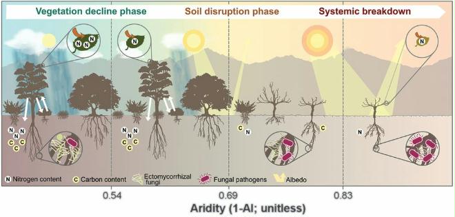
Earth’s dryland ecosystem covers 45% of the world’s surface and is home to around a third of its population who depend on these areas for their food and water.
This study found that as aridity increases, dryland ecosystems undergo a series of abrupt changes. This results first in drastic reductions in the capacity of plants to fix carbon from the atmosphere, then substantial declines of soil fertility, drought-tolerant plants replace food crops, and finally vegetation disappears under the most arid and extreme conditions and turns into a desert.
As aridification grows worse, the land becomes more vulnerable to erosion, soil biota maintaining the ecosystem decline, pathogens increase, crops fail.
More than 20% of land may cross these thresholds by 2100 due to climate change.
Climate disruptions to agricultural production have increased in the past 40 years and are projected to increase over the next 25 years. By 2050 and beyond, these impacts will be increasingly negative on most crops and livestock.
Many agricultural regions will experience declines in crop and livestock production from increased stress due to weeds, diseases, insect pests, and other climate change induced stresses.
Current loss and degradation of critical agricultural soil and water assets due to increasing extremes in precipitation will continue to challenge both rain-fed and irrigated agriculture
The rising incidence of weather extremes will have increasingly negative impacts on crop and livestock productivity because critical thresholds are already being exceeded.
Agriculture has been able to adapt to recent changes in climate; however, increased innovation will be needed to ensure the rate of adaptation of agriculture and the associated socioeconomic system can keep pace with climate change over the next 25 years.
Climate change effects on agriculture will have consequences for food security, both in the U.S. and globally, through changes in crop yields and food prices and effects on food processing, storage, transportation, and retailing. Adaptation measures can help delay and reduce some of these impacts.
The United States produces nearly $330 billion per year in agricultural commodities, with livestock accounting for half of that value. Production of all commodities will be vulnerable to direct impacts (from changes in crop and livestock development and yield due to changing climate conditions and extreme weather events) and indirect impacts (through increasing pressures from pests and pathogens that will benefit from a changing climate). Crop production projections often fail to consider the indirect impacts from weeds, insects, and diseases that accompany changes in both average trends and extreme events, which can increase losses significantly.
Rising average temperatures will increase crop water demand, increasing the rate of water use by the crop. Higher temperatures are projected to increase both evaporative losses from land and water surfaces and transpiration losses (through plant leaves) from non-crop land cover, potentially reducing annual runoff and streamflow for a given amount of precipitation.
By mid-century, when temperature increases are projected to be between 1.8°F and 5.4°F and precipitation extremes are further intensified, yields of major U.S. crops and farm profits are expected to decline. There have already been detectable impacts on production due to increasing temperatures.
One critical period in which temperatures are a major factor is the pollination stage; pollen release is related to development of fruit, grain, or fiber. Exposure to high temperatures during this period can greatly reduce crop yields and increase the risk of total crop failure. Plants exposed to high nighttime temperatures during the grain, fiber, or fruit production period experience lower productivity and reduced quality. These effects have already begun to occur; high nighttime temperatures affected corn yields in 2010 and 2012 across the Corn Belt. With the number of nights with hot temperatures projected to increase as much as 30%, yield reductions will become more prevalent.
Plants have specific temperature tolerances, and can only be grown in areas where their temperature thresholds are not exceeded. As temperatures increase over this century, crop production areas may shift to follow the temperature range for optimal growth and yield of grain or fruit. Temperature effects on crop production are only one component; production over years in a given location is more affected by available soil water during the growing season than by temperature, and increased variation in seasonal precipitation, coupled with shifting patterns of precipitation within the season, will create more variation in soil water availability.
Increasing temperatures cause cultivated plants to grow and mature more quickly. Crops, such as cereals, would grow more quickly, meaning less time for the grain itself to mature, reducing productivity. But because the soil may not be able to supply nutrients at required rates for faster growing plants, plants may be smaller, reducing grain, forage, fruit, or fiber production.
In vegetables, exposure to temperatures in the range of 1.8°F to 7.2°F above optimal moderately reduces yield, and exposure to temperatures more than 9°F to 12.6°F above optimal often leads to severe if not total production losses.
Temperature and precipitation changes will include an increase in both the number of consecutive dry days (days with less than 0.01 inches of precipitation) and the number of hot nights. The western and southern parts of the nation show the greatest projected increases in consecutive dry days, while the number of hot nights is projected to increase throughout the U.S. These increases in consecutive dry days and hot nights will have negative impacts on crop and animal production. High nighttime temperatures during the grain-filling period (the period between the fertilization of the ovule and the production of a mature seed in a plant) increase the rate of grain-filling and decrease the length of the grain-filling period, resulting in reduced grain yields. Exposure to multiple hot nights increases the degree of stress imposed on animals resulting in reduced rates of meat, milk, and egg production.
Climate change poses a major challenge to U.S. agriculture because of the critical dependence of the agricultural system on climate and because of the complex role agriculture plays in rural and national social and economic systems (Figure 6.2). Climate change has the potential to both positively and negatively affect the location, timing, and productivity of crop, livestock, and fishery systems at local, national, and global scales. It will also alter the stability of food supplies and create new food security challenges for the United States
Over time, climate change is expected to increase the annual variation in crop and livestock production because of its effects on weather patterns and because of increases in some types of extreme weather events.
Each crop species has a temperature range for growth, along with an optimum temperature.9 Plants have specific temperature tolerances, and can only be grown in areas where their temperature thresholds are not exceeded. As temperatures increase over this century, crop production areas may shift to follow the temperature range for optimal growth and yield of grain or fruit. Temperature effects on crop production are only one component; production over years in a given location is more affected by available soil water during the growing season than by temperature, and increased variation in seasonal precipitation, coupled with shifting patterns of precipitation within the season, will create more variation in soil water availability. The use of a model to evaluate the effect of changing temperatures
Key Message: Extreme Precipitation and Soil Erosion
Current loss and degradation of critical agricultural soil and water assets due to increasing extremes in precipitation will continue to challenge both rainfed and irrigated agriculture unless innovative conservation methods are implemented. Wind erosion could also increase in areas with persistent drought because of the reduction in vegetative cover.
Several processes act to degrade soils, including erosion, compaction, acidification, salinization, toxification, and net loss of organic matter. Several of these processes, particularly erosion, will be directly affected by climate change. Rainfall’s erosive power is expected to increase as a result of increases in rainfall amount in northern portions of the United States, accompanied by further increases in precipitation intensity. Projected increases in rainfall intensity that include more extreme events will increase soil erosion in the absence of conservation practices. Precipitation and temperature affect the potential amount of water available, but the actual amount of available water also depends on soil type, soil water holding capacity, and the rate at which water filters through the soil.
Iowa is the nation’s top corn and soybean producing state. These crops are planted in the spring. Heavy rain can delay planting and create problems in obtaining a good stand of plants, both of which can reduce crop productivity. In Iowa soils with even modest slopes, rainfall of more than 1.25 inches in a single day leads to runoff that causes soil erosion and loss of nutrients and, under some circumstances, can lead to flooding. Figure 6.9 shows the number of days per year during which more than 1.25 inches of rain fell is increasing.
A few of the ecosystem services provided by soils include:
the provision of food
wood
fiber (i.e. cotton)
raw materials
flood mitigation
recycling of wastes
biological control of pest
regulation of carbon and other heat-trapping gases
physical support for roads and buildings
cultural and aesthetic values
Productive soils are characterized by levels of nutrients necessary for the production of healthy plants, moderately high levels of organic matter, a soil structure with good binding of the primary soil particles, moderate pH levels, thickness sufficient to store adequate water for plants, a healthy microbial community, and the absence of elements or compounds in concentrations that are toxic for plant, animal, and microbial life.
Erosion is managed through maintenance of cover on the soil surface to reduce the effect of rainfall intensity. Studies have shown that a reduction in projected crop biomass (and hence the amount of crop residue that remains on the surface over the winter) will increase soil loss.
Key Message: Weeds, Diseases, and Pests
Many agricultural regions will experience declines in crop and livestock production from increased stress due to weeds, diseases, insect pests, and other climate change induced stresses.
The growth of atmospheric CO2 concentrations has a disproportionately positive impact on several weed species. This effect will contribute to increased risk of crop loss due to weed pressure.
Weeds, insects, and diseases already have large negative impacts on agricultural production, and climate change has the potential to increase these impacts. Current estimates of losses in global crop production show that weeds cause the largest losses (34%), followed by insects (18%), and diseases (16%). Further increases in temperature and changes in precipitation patterns will induce new conditions that will affect insect populations, incidence of pathogens, and the geographic distribution of insects and diseases. Increasing CO2 boosts weed growth, adding to the potential for increased competition between crops and weeds. Several weed species benefit more than crops from higher temperatures and CO2 levels.
One concern involves the northward spread of invasive weeds like privet and kudzu, which are already present in the southern states. Changing climate and changing trade patterns are likely to increase both the risks posed by, and the sources of, invasive species. Controlling weeds costs the U.S. more than $11 billion a year, with most of that spent on herbicides. Both herbicide use and costs are expected to increase as temperatures and CO2 levels rise. Also, the most widely used herbicide in the United States, glyphosate, loses its efficacy on weeds grown at CO2 levels projected to occur in the coming decades. Higher concentrations of the chemical and more frequent sprayings thus will be needed, increasing economic and environmental costs associated with chemical use.
Insects are directly affected by temperature and synchronize their development and reproduction with warm periods and are dormant during cold periods. Higher winter temperatures increase insect populations due to overwinter survival and, coupled with higher summer temperatures, increase reproductive rates and allow for multiple generations each year. An example of this has been observed in the European corn borer (Ostrinia nubialis) which produces one generation in the northern Corn Belt and two or more generations in the southern Corn Belt. Changes in the number of reproductive generations coupled with the shift in ranges of insects will alter insect pressure in a given region.
Key Message: Heat and Drought Damage
The rising incidence of weather extremes will have increasingly negative impacts on crop and livestock productivity because critical thresholds are already being exceeded.
Climate change projections suggest an increase in extreme heat, severe drought, and heavy precipitation. Extreme climate conditions, such as dry spells, sustained droughts, and heat waves all have large effects on crops and livestock. The timing of extreme events will be critical because they may occur at sensitive stages in the life cycles of agricultural crops or reproductive stages for animals, diseases, and insects. Extreme events at vulnerable times could result in major impacts on growth or productivity, such as hot-temperature extreme weather events on corn during pollination. By the end of this century, the occurrence of very hot nights and the duration of periods lacking agriculturally significant rainfall are projected to increase. Recent studies suggest that increased average temperatures and drier conditions will amplify future drought severity and temperature extremes. Crops and livestock will be at increased risk of exposure to extreme heat events. Projected increases in the occurrence of extreme heat events will expose production systems to conditions exceeding maximum thresholds for given species more frequently.
California’s Wine, Fruit, & Nut production will begin declining as soon as 2050
In fact, it’s already happening. In 2000, the number of chilling hours in some regions was 30% lower than in 1950. A warmer climate will affect growing conditions, and the lack of cold temperatures may threaten perennial crop production (Figure 6.6), which have a winter chilling requirement (expressed as hours when temperatures are between 32°F and 50°F) ranging from 200 to 2,000 cumulative hours. Yields decline if the chilling requirement is not completely satisfied, because flower emergence and viability is low. Projections show that chilling requirements for fruit and nut trees in California will not be met by the middle to the end of this century.
Impacts on Animal Production
Animal agriculture is a major component of the U.S. agriculture system. Changing climatic conditions affect animal agriculture in four primary ways: 1) feed-grain production, availability, and price; 2) pastures and forage crop production and quality; 3) animal health, growth, and reproduction; and 4) disease and pest distributions. The optimal environmental conditions for livestock production include temperatures and other conditions for which animals do not need to significantly alter behavior or physiological functions to maintain relatively constant core body temperature.
Optimum animal core body temperature is often maintained within a 4°F to 5°F range, while deviations from this range can cause animals to become stressed. This can disrupt performance, production, and fertility, limiting the animals’ ability to produce meat, milk, or eggs. In many species, deviations in core body temperature in excess of 4°F to 5°F cause significant reductions in productive performance, while deviations of 9°F to 12.6°F often result in death. For cattle that breed during spring and summer, exposure to high temperatures reduces conception rates. Livestock and dairy production are more affected by the number of days of extreme heat than by increases in average temperature. Elevated humidity exacerbates the impact of high temperatures on animal health and performance.
Animals respond to extreme temperature events (hot or cold) by altering their metabolic rates and behavior. Increases in extreme temperature events may become more likely for animals, placing them under conditions where their efficiency in meat, milk, or egg production is affected. Projected increases in extreme heat events will further increase the stress on animals, leading to the potential for greater impacts on production. Meat animals are managed for a high rate of weight gain (high metabolic rate), which increases their potential risk when exposed to high temperature conditions. Exposure to heat stress disrupts metabolic functions in animals and alters their internal temperature when exposure occurs. Exposure to high temperature events can be costly to producers, as was the case in 2011, when heat-related production losses exceeded $1 billion.
Livestock production faces additional climate change related impacts that can affect disease prevalence and range. Regional warming and changes in rainfall distribution have the potential to change the distributions of diseases that are sensitive to temperature and moisture, such as anthrax, blackleg, and hemorrhagic septicemia, and lead to increased incidence of ketosis, mastitis, and lameness in dairy cows.
Goats, sheep, beef cattle, and dairy cattle are the livestock species most widely managed in extensive outdoor facilities. Within physiological limits, animals can adapt to and cope with gradual thermal changes, though shifts in thermoregulation may result in a loss of productivity. Lack of prior conditioning to rapidly changing or adverse weather events, however, often results in catastrophic deaths in domestic livestock and losses of productivity in surviving animals.
Key Message: Rate of Adaptation
Agriculture has been able to adapt to recent changes in climate; however, increased innovation will be needed to ensure the rate of adaptation of agriculture and the associated socioeconomic system can keep pace with climate change over the next 25 years.
In the longer term existing adaptive technologies will likely not be sufficient to buffer the impacts of climate change without significant impacts to domestic producers, consumers, or both. Limits to public investment and constraints on private investment could slow the speed of adaptation. Adaptation may also be limited by the availability of inputs (such as land or water), changing prices of other inputs with climate change (such as energy and fertilizer), and by the environmental implications of intensifying or expanding agricultural production.
In addition to regional constraints on the availability of critical basic resources such as land and water, there are potential constraints related to farm financing and credit availability in the U.S. and elsewhere. Research suggests that such constraints may be significant, especially for small family farms with little available capital.
Farm resilience to climate change is also a function of financial capacity to withstand increasing variability in production and returns, including catastrophic loss. As climate change intensifies, “climate risk” from more frequent and intense weather events will add to the existing risks commonly managed by producers, such as those related to production, marketing, finances, regulation, and personal health and safety factors. The role of innovative management techniques and government policies as well as research and insurance programs will have a substantial impact on the degree to which the agricultural sector increases climate resilience in the longer term.
Key Message: Food Security
Climate change effects on agriculture will have consequences for food security, both in the U.S. and globally, through changes in crop yields and food prices and effects on food processing, storage, transportation, and retailing.
Food security includes four components: availability, stability, access, and utilization of food. Following this definition, in 2011, 14.9% of U.S. households did not have secure food supplies at some point during the year, with 5.7% of U.S. households experiencing very low food security.
In addition to altering agricultural yields, projected rising temperatures, changing weather patterns, and increases in frequency of extreme weather events will affect distribution of food- and water-borne diseases as well as food trade and distribution. This means that U.S. food security depends not only on how climate change affects crop yields at the local and national level, but also on how climate change and changes in extreme events affect food processing, storage, transportation, and retailing, through the disruption of transportation as well as the ability of consumers to purchase food. And because about one-fifth of all food consumed in the U.S. is imported, our food supply and security can be significantly affected by climate variations and changes in other parts of the world. The import share has increased over the last two decades, and the U.S. now imports 13% of grains, 20% of vegetables (much higher in winter months), almost 40% of fruit, 85% of fish and shellfish, and almost all tropical products such as coffee, tea, and bananas. Climate extremes in regions that supply these products to the U.S. can cause sharp reductions in production and increases in prices.
In an increasingly globalized food system with volatile food prices, climate events abroad may affect food security in the U.S. while climate events in the U.S. may affect food security globally. The globalized food system can buffer the local impacts of weather events on food security, but can also increase the global vulnerability of food security by transmitting price shocks globally.
Senate 113-245. February 14, 2013. Drought, fire and freeze: the economics of disasters for America’s agricultural producers. U.S. Senate hearing.
Excerpts from this 195-page document follow.
DEBBIE STABENOW, MICHIGAN. Nobody feels the effect of weather disasters more than our nation’s farmers and ranchers, as we all know, whose livelihoods depend on getting the right amount of rain, the right amount of sunshine, getting it all together the right way at the right time. All too frequently, an entire season’s crop can be lost, as we know. Or an entire herd must be sent to slaughter due to the lack of feed.
The year 2012 was a year of unprecedented destruction, from drought, freezes, wildfires, hurricanes, and tornadoes, including the tornadoes that hit Mississippi and other parts of the South last weekend, and my heart goes out to all the survivors of those devastating storms. Our country experienced two of the most destructive hurricanes on record last year, Isaac and Sandy. We experienced the warmest year on record ever in the contiguous United States, which, coupled with the historic drought, produced conditions that rivaled the Dust Bowl. Wildfires raged in the West. In the Upper Midwest and Northeast, warm weather in February and March caused trees to bloom early, resulting in total fruit destruction when temperatures dropped down to the 20s again in April, and we certainly were hit hard with that in Michigan. California and Arizona experienced a freeze just last month, threatening citrus, strawberries, lettuce, and avocados. We learned last week that our cattle herd inventories are the lowest in over six decades, which has had broad-ranging impacts, including job losses in rural communities as processing facilities and feedlots idle.
The drought has left many of our waterways with dangerously low water levels. Lake Michigan, Lake Huron have hit their all- time lowest water levels. Barge traffic on the Mississippi, our most vital waterway has nearly ground to a halt. We have seen major disruptions and increased transportation costs for commodities and fertilizers. Today, we will hear from officials at the National Oceanic and Atmospheric Administration, NOAA, and the Department of Agriculture about the disasters we faced last year. We also will hear directly from those affected by these disasters. Thanks to our successful Crop Insurance Program, many farmers will be able to recover their losses. For those farmers who did not have access to crop insurance or the other risk management tools we worked so hard to include in our Senate-passed farm bill, the future is less certain. Unfortunately, instead of a farm bill that gave those farmers certainty, we ended up with a partial extension that creates the haves and haven’ts. Low crop producers that participate in crop insurance not only get assistance from crop insurance, which is essential, but some will continue to receive direct payments, as well, regardless if they have a loss. Meanwhile, many livestock producers and specialty crop growers who suffered substantial losses will not receive any assistance.
We all know that farming is the riskiest business in the world and altogether employs 16 million Americans.
ROGER PULWARTY, Director, National Integrated Drought Information System, NATIONAL OCEANIC & ATMOSPHERIC ADMINISTRATION, BOULDER, COLORADO
Drought is a pallet of the American experience, from the Southwest in the 13th century to the events of the 1930s and the 1950s to the present. From 2000 to 2010, the annual average land area affected by drought in the United States was 25 percent. Prior to the 2000s, this number stood at 15 percent. 2012 ended as one of the driest years on record, having had five months in which over 60 percent of the country was in moderate to extreme drought. It was also the warmest year on record. Only 1934 had more months with over 60 percent of the U.S. in moderate to severe drought. 1934 was also a warm year.
Drought conditions continue across much of the nation. According to one estimate, the cost of the 2012 drought is in excess of $35 billion, based on agriculture alone.
However, it is important to note the drought-related impacts cross a broad spectrum, from energy, tourism, and recreation in the State of Colorado where I live, to wildfire impacts. According to the National Interagency Fire Center in Boise, over nine million acres were burned last year, which had only happened twice before in the record, 2006 and 2007, since 1960. Low river levels also threaten commerce on the vital Mississippi shipping lanes, affecting transportation of agricultural products. As many of you know, half of the transport on the Mississippi is agriculturally based.
An important feature of conditions in 2012 was the persistence of the area of dryness and warm temperatures, the magnitude of the extremes, and the large area they encompassed.
Twenty-twelve began with about 32 percent of the U.S. in moderate to exceptional drought. The drought reintensified in May, and you can see a jump in the figure there. And by the end of August, the drought had expanded to cover 60 percent of the country, from the Central Rockies to the Ohio Valley and the Mexican to the Canadian borders. Several States had record dry seasons, including Arkansas, Kansas, Nebraska and South Dakota.
The drought years of 1955 and 1956 have the closest geographical pattern to what we have seen to date, and the year 1998, now the second-warmest year on record, and 2006, the third-warmest year on record, have the closest temperature pattern to what we see.
So as of this morning, we have released the U.S. Drought Monitor that gives you present conditions, which people have in front of them. And what we are pointing out in this case is the drought continues across many parts of the Midwest and the West. The physical drivers of drought are linked to sea surface temperatures in the Tropical Pacific and Atlantic Oceans.
As you can see from the last figure on the U.S. Drought Monitor, a dry pattern is expected over the upcoming three months across the South and the Midwest. Prospects are limited for improvement in drought conditions in California, Nevada, and Western Arizona. Drought development and persistence is forecasted for Texas by the end of April. The drought and warm temperatures in the Midwest are firmly entrenched into February, placing a greater need for above-normal spring rains if the region is to recover. This area is now becoming the epicenter of the 2013 drought. Despite some relief, much of the Appalachicola-Chattahoochee-Flint River Basin remain under extreme drought conditions, including low ground water levels, and Georgia is now in its driest two-year period on record.
JOE GLAUBER, CHIEF ECONOMIST, U.S. DEPARTMENT OF AGRICULTURE, WASHINGTON, DC
Row crop producers have generally fared well, despite the adverse weather, in large part due to higher prices and protection from the Federal Crop Insurance Program, which has helped offset many of the yield losses. For uninsured producers, or producers of crops for which insurance is unavailable, however, crop losses have had a more adverse effect. Livestock producers experienced high feed costs and poor pasture conditions this year with limited programs to fall back on, particularly since key livestock disaster programs authorized under the 2008 farm bill are currently unfunded.
What had started out as a promising year for U.S. crop production, with favorable planting conditions supporting high planted acreage and expectations of record or near- record production turned into one of the most unfavorable growing seasons in decades. Crop production estimates for several major crops declined throughout the summer. By January 2013, final production estimates for corn were down almost 28 percent from our May projections. Sorghum was down 26 percent, while soybeans fell about six percent over the same period.
As a result, prices for grains and oil seeds soared to record highs in the summer. Higher prices and crop insurance indemnity payments helped offset crop losses for many rural crop producers. Roughly 85 percent of corn, wheat, and soybean area, almost 80 percent of rice area, and over 90 percent of cotton area is typically enrolled in the Crop Insurance Program, and for those of you who were around back in 1988, this contrasts sharply with what the experience was in 1988 when we had this massive drought in the Midwest. At that time, only about 25 percent of the area, insurable area, was enrolled in the program. So, again, very, very strong participation has helped offset those losses.
As of February 11, just this Monday, about $14.2 billion in indemnity payments have been made to producers of 2012 crops suffering crop or revenue losses. We think that these indemnity payments will likely go higher. They could be as high as 16 or 17 billion dollars before we are done.
On the other hand, looking at the livestock, dairy, and poultry producers, they are facing very high feed costs for most—they faced very high feed costs for most of 2012, and the high prices are likely to persist through much of 2013 until new crops become available in the fall. And in addition to these high feed costs, cattle producers have been particularly hard hit by poor pasture conditions and a poor hay crop. Almost two- thirds of the nation’s pasture and hay crops were in drought conditions, with almost 60 percent of pasture conditions rated poor or very poor for most of July, August, and September 2012. December 1 stocks for hay were at their lowest level since 1957.
The U.S. cattle and calf herd, as was mentioned in your statement, is at its lowest level since 1952. Dryness in the Southern Plains has persisted for over two years and resulted in large liquidation in cattle numbers. The January 1 NASS Cattle Report indicated that total cattle and calf numbers in Kansas, Oklahoma, and Texas alone declined by 3.4 million head between 2011 and 2013. The reduction is a 13.6 percent decline and almost equals the net decline in the U.S. herd over the same period. Likewise, dairy producers have faced high feed costs and poor pasture conditions, and higher temperatures during the summer also adversely affected milk production.
Net cash income is forecast lower in 2013 for all livestock, dairy, and poultry sector. Feed costs make up 51 percent of expenses for dairy, about 20 percent for beef cattle, 42 percent for hogs, and 35 percent for poultry farm businesses.
Major concerns related to persistent drought conditions remain. Fifty-nine percent of wheat area, the winter wheat area, 69 percent of cattle production, and 59 percent of hay acreage remains under drought conditions. Forty-three percent of the winter wheat production is located in areas under extreme or exceptional drought conditions, down only slightly from the 51 percent in August.
Chairwoman STABENOW. How long before we are going to have crop insurance available for specialty crop growers?
Mr. GLAUBER. I think we have made some improvements there. As you know, I sit on the Federal Crop Insurance Board. We have seen several products, new products that have come in that have extended crop insurance to some specialty crops. We have made some changes, for example, in the cherry policy with a revenue product. I think the overall liability for specialty crops right now is around 10 to 13 billion dollars. Certainly, we would like to see that improved. The difficulty is that with a lot of these crops, they are very small with not a lot of producers, and sometimes some of the producers are not interested in crop insurance. Now, what we have seen over the last five years, ten years, which is very different than, I would say, 15 years ago, is the fact that a lot of producers now are interested in developing these products.
Our major issue, as you know, in the Midwest and the Southwest, in particular, the Colorado Basin, is that we are having back- to-back dry years, and a third year of that puts our systems completely under stress. The forecast for this season is that, in fact, we are projecting drier conditions.
Senator KLOBUCHAR. Mississippi River transportation is my next question. In 2012, as you know, the barge traffic on the Mississippi was greatly impacted by the drought. It was more difficult to transport grain abroad and more farm inputs up-river to our farmers in Minnesota. We were very scared at the end of the year they were actually going to have to stop barge traffic. Could you talk about that a little and how this could impact our ability to stay competitive, as so many agriculture products go down the Mississippi?
Mr. GLAUBER. Yes. We, too, were very concerned with it because it looked like, particularly late December, early January, that there would be a halt in traffic. Now, understand, the upper part of the Mississippi, as you well know, you stop shipping because of the winter weather. But I think there were a couple of good things. One, the best thing, is that we got rain. The Corps was able to go in and clear out some of the disruptions in the river and then we got adequate rain and barge traffic is moving very well. I will say this. Because of the lower corn harvest and lower soybean harvest and the fact that so much more grain is going to China, it was probably less stress than it might have been under, say, 15 years ago. But, still, the best news is that we have adequate water.
Senator KLOBUCHAR. It is good, but it was a close call and I think it is something that we have to prepare better for next time and have a plan in place. Drought-resistant seeds—what efforts is the USDA taking to speed the adoption of such drought-hardy varieties developed using biotech or conventional breeding?
Mr. GLAUBER. Most of the breeding for seed breeding is in private hands these days. They do it better. There are a lot of profits to be made in that industry and they are working very hard. My understanding is, is that we should be seeing some disaster-resistant, purely disaster-resistant strains come on the market just in the next few years. We know upstream, as well, about 20 percent of what comes into the basin is coal and 20 percent is about fertilizers, as well.
Senator ROBERTS. We have got two years of sustained drought and another one coming, according to our renowned forecaster here. But Kansas producers, once again, put seeds in the ground. Many will once again fire up their tractor and their planter in another six weeks. They manage their risk and protect their operations from Mother Nature’s destruction through the purchase of crop insurance.
Unfortunately, livestock producers do not have a similar safety net. However, with the support of Secretary Vilsack last year, the Department authorized the emergency haying and grazing of Conservation Reserve Program acres in all Kansas counties, including the emergency grazing on CP-25 for the first time. You do not do that unless you have a very, very serious problem.
According to USDA reports last year, over 9,000 emergency haying and grazing contracts allowed haying and grazing on over 470,000 acres in Kansas, that’s a lot of acres. But as we continue to experience what we have experienced in the 1950s and back in the 1930s, what considerations has the Department given to allowing emergency haying and grazing of CRP acres for 2013??
Mr. GLAUBER. A lot of these producers have been hanging on with very, very tight or negative margins. And again, I cited these numbers. Over three million, three-and-a-half million head down from just two years ago in your region of the country. And so it is very critical. I think any help that we can get to the producers to help them make it through to better prices, we will be working with your office on that.
Senator ROBERTS. As you know, many ranchers simply culled their herds and lost their genetics and many are out of business. Northwest Kansas producers irrigating from the Ogallala Aquifer, they must work to conserve their water, but current RMA practices do not have a middle ground between fully irrigated and dry land practices and we need a mechanism to allow limited irrigation to be fairly rated.
Senator BENNET. —we have now had two years in a row, and it sounds like we are going to have a third year of drought in our region. And I wonder if you could talk about the specific challenges that NOAA projects for producers in the water-scarce Western region of our country.
Mr. PULWARTY. I hope I am wrong, as well. The State of Colorado, as you know, in the Front Range, where I live and others do, we get 30 to 40 percent of our water from the Colorado Basin itself. The Colorado Basin came in at 44 percent in the previous water year. So far, the fall snow pack has not been as significant as we would like it. In some places, it is 40, some places 60%, and we hope that picks up in March and April.
However, right now, based on what is happening in the Pacific Ocean and the Atlantic Oceans, we are not projecting an improved set of conditions in those basins, the Upper Basin, including the San Juan and places like that.
The area in terms of the basin is experiencing some lower precipitation and snow pack, and it is also experiencing a combination of high temperatures, however driven. Something else that is happening in that basin has to do with some of our rural communities, where there is rain-fed agriculture.
the combination of temperature and drought is actually creating the die-off of key vegetation that holds our soils together. And the result, then, is dust storms, dust on snow, which lets the runoff and melt occur even earlier than we are accustomed to managing it.
From that standpoint, and looking into the future, while we are seeing some improvement in the lower Colorado Basin—Arizona, Southern California, Nevada—we are expecting that to be short- lived into April. From the standpoint of the Upper Basin, and again, I hope I am, in fact, wrong, we are not projecting significant new inputs of snow unless we get heavy rainfall events later in the spring.
One of the reasons why that is the case is when it has been dry for a year before, even when you get significant snow pack, a lot of that disappears because the soil just picks it up. In 2005, we had 100 percent of snow pack, but the runoff was 70 percent of what we expected because the springtime had been warm.
The Colorado is now in its second longest ten-year period of low flows on record. If we average over the last ten years, the flow has been at average or less, and this is in an already over-allocated system, as you know better than I do.
The issue concerning the basin, where 30 million people live and where we have seven States reliant on the water, is very much at the edge. The demand exceeded supply about ten years ago, so it does not take a major drought to put us into areas of contention.
And to be perfectly honest, given the uncertainty, certainly, there are issues in introducing drought-resistant crops. There are issues in introducing risk pooling and insurance. But where the Conservation Reserve Programs come in is the admission that we are uncertain about the future, that it leaves us the flexibility to manage for the pieces that we are uncertain about. And I think that is the richest contribution from the standpoint of an understand what the weather incline is doing, naturally or otherwise, and then what the buffers in our system supply.
Senator COWAN. We also need to be thinking about new threats that our farmers and fishermen are facing. The climate change and more frequent and intense extreme weather events threaten our agricultural economy, and I am pleased that the committee is discussing this important issue today.
According to the Climate Vulnerability Initiative, the U.S. is among the top ten countries that will be most adversely affected by desertification and sea level risk, and this does not bode well for either our farmers or fishermen.
Senator BAUCUS. It is a real honor for me to introduce Leon LaSalle. Leon is a Native American rancher. The real deal, several generations. His grandfather, Frank Billy, is one of the first to found the ranch on the Chippewa Cree Reservation of Montana. It actually is part of the Rocky Boys Reservation. We have got seven reservations in Montana. Leon and his family are real stalwarts, and one of the reservations is Rocky Boys and the Chippewa Cree are the Tribal members in that reservation. They raise Black Angus around the Bears Paw Mountains between Rocky Boys, up around Havre, Montana. It is sort of a real standout, that is, as a landmark in our State. We are very proud of it. Leon was featured in a book. The book was called Big Sky Boots. It is the working seasons of a Montana cowboy. He has a great quote in that book. He said he thinks there is a growing disconnect between the general public and agriculture producers. Well, Leon, I have got to tell you, the same thing is true in Washington, D.C. There is a disconnect between the people here and the people who represent the rest of the country, and maybe you can kind of help connect those dots a little bit here when it comes time for you to testify. We are really very honored to have you here because you are a great credit to the Tribe and to the State of Montana and your industry. Leon is also on the Board of Directors of the Montana Stockgrowers and one of the guiding lights there,
LEON LASALLE, RANCHER, HAVRE, MONTANA
We have installed numerous conservation practices specifically designed to preserve and protect our natural resources. Even though we have implemented these conservation measures, there are times when my family’s ranch has been struck so hard by weather- related disasters that we have sought economic assistance. The Federal Livestock Disaster Programs have been that assistance.
The Native American Livestock Feed Program is a great example of a program that helped when feed was short. In drought years, when there is little or no hay to feed our livestock, ranchers like me must purchase hay at a premium. Sometimes by the time the hay reaches the ranch, the freight is more than the cost of the hay itself.
These programs provide the only financial relief available when a rancher was faced with loss of livestock or forage to feed them. There is no insurance for catastrophic livestock losses, such as those experienced by Southeastern Montana ranchers during the horrific wildfires of 2012.
I have helped neighbors prepare applications for LIP, and on one sad occasion, I participated as a third-party witness when several cattle fell through the ice and drowned while trying to shelter themselves from a stinging Montana blizzard.
Mother Nature throws a variety of natural events in the path of a Montana rancher. Our weather is uncertain, sometimes severe. We find our markets are even vulnerable to the effects of drought, as well. Drought has reduced the number of cattle available, and processing facilities have closed as a result, thus affecting our price. If weather and markets are not the issue, then many of my fellow ranchers are challenged by the ever- increasing predator losses.
ANNGIE STEINBARGER, FARMER, EDINBURGH, INDIANA
we now farm 1,500 acres of corn and soybeans as well as a small cow-calf operation in the State. We find our association with various farm organizations, such as the Indiana Soybean Alliance, invaluable to the success of our operation. The Indiana Soybean Alliance is an arm of the American Soybean Association, a trade organization that represents our nation’s 600,000 soybean farmers on national and international policy issues.
It has always been our dream to farm. My husband and I both knew that the only way to make our dreams a reality were to save our pennies and work off-farm incomes in hope that, one day, my father would give us the opportunity to participate in the farming operation. Mike worked in the seed, tile ditching, and bulk milk transport business while I worked in fertilizer, chemical, and crop insurance businesses.
We started farming 600 acres and have increased the operation to 1,500 acres. Roughly one-half of our acres are on a share arrangement with our landlords. We continue to work off- farm, as it is still not self-supporting. Mike sold the milk truck to buy a school bus and I continue to work in the crop insurance and do the farm recordkeeping.
To manage our thin, light soil types, we started our farming operation employing conservation tillage techniques, using such programs as CRP and NRCS cost share funding. To this day, we are still advocates of no-till farming as a way to preserve our soil and maintain soil moisture. As a result of our conservation efforts, our average yields are 150 bushels of corn and 50 bushels of soybeans.
Our best corn was on the farm with the pivot. Under the pivot, it was 200 bushels to the acre. And outside of the pivot, ten. Needless to say, there was not anything to put in the grain bins. Due to the drought and heat, the grain quality was very poor and we even shipped our grain that was going to be fed for livestock.
The number one barrier to increasing our yields is the lack of water. Dry weather in the months of July and August always limit our yield potential. We find crop insurance an effective tool in managing risk when we experience these weather events. We began using crop insurance in 1991 as a way to maintain our cash flow and prevent us from having to borrow money. I actually have lost money over buying crop insurance over the last 20- year time span. It was not until the last two drought years that it actually paid for us to have crop insurance.
JEFF SEND, CHERRY FARMER, LEELANAU, MICHIGAN
I grew up working my grandfather’s 40 acres. Now, my wife and I, Anita, farm 800 acres of sweet and tart cherries. Putting some of the land into the Federal Farm and Ranch Land Protection Program is one of the tools we use to expand our operation. Our youngest daughter and her husband work with us and they someday hope to take over the farm. I also have managed a receiving station for 37 years. I have a working relationship with 35 growers who bring me cherries to be weighed, inspected, shipped to ten different processors in Michigan, Wisconsin, and the State of New York that I work with. I currently am serving as Vice Chair of the Cherry Marketing Institute Board. CMI is a national organization for tart cherry farmers. I am also a Vice Chair of the National Cherry Growers and Industries Foundation, which is a sweet cherry organization. Year in and year out, Michigan produces 75 percent of the United States tart cherries. However, that was not the case in 2012. Last year was the most disastrous year I and the cherry industry have ever experienced. Our winter was much warmer than normal, with little snow and ice on the Great Lakes. In mid-March, there were seven days of 80-degrees temperatures, which is unheard of in Northern Michigan. Cherry trees began to come out of dormancy and began to grow. This left them completely vulnerable to the next 13 freezes in April. This extreme weather in Michigan was one of the worst disasters we had ever seen. Sweet cherries endured freezes slightly better than tart cherries. But to top things off, we were hit with a worst case bacterial canker I had ever seen. There is no treatment for this disease, which affects the fruit buds.
In Michigan, we have the capacity to grow 275 million pounds of tart cherries. In 2012, our total was 11.6 million pounds.
There is no tart cherry insurance available at all for our industry, so my fellow growers and I had no risk management tool to get through this very difficult year. NAP insurance is available, but the policy starts at 50% loss and then pays out only 50% of that number. Farmers are left with only about 25% of coverage, and there is a $100,000 cap. This does not come close to covering our expenses. My costs on my farm alone are between three-quarters and a million dollars.
Tree fruits must be maintained whether there is a crop or not on them. You carry on with the same practices in order to keep them healthy. So expenses remain the same. Imagine working for a year-and-a-half with no paycheck and still having the same expenses.
I worry about our young farmers, who haven’t built up any equity. No income with all the same expenses is formula for disaster. There needs to be something to help farmers stay in business when natural disaster hits. A few days that we have no control over can put us out of business.
BEN E. STEFFEN, FARMER, STEFFEN AG, INC., HUMBOLDT, NEBRASKA
My family, our employees, and I produce milk, corn, soybeans, wheat, and hay on our farm at Humboldt in Southeast Nebraska. We milk 135 cows on 1,900 acres of non-irrigated dryland farm, and I have family members at home right now caring for and feeding animals so that I can be here today.
My family, our employees, and I produce milk, corn, soybeans, wheat, and hay on our farm at Humboldt in Southeast Nebraska. We milk 135 cows on 1,900 acres of non-irrigated dryland farm, and I have family members at home right now caring for and feeding animals so that I can be here today. This nation has benefited from a food supply that is plentiful, inexpensive, and of the highest quality, and securing that food supply for the future is clearly a responsible public policy. Facing a growing world population, it is a moral imperative. The impact of fire and drought has hit our farming operation and those of our neighbors. The price of high-quality dairy hay has gone up by 50 percent, and the price of lower- quality hay suitable for beef animals has more than doubled. While we appreciated last year’s release of Conservation Reserve Program acres for emergency haying and grazing, we would like to see efforts made for an earlier release date for those acres. This would dramatically improve the quality and the quantity of those forages.
My neighbors in Western Nebraska have been dealt a particularly hard blow by wildfires, and nearly 400,00 acres, approximately half the State—equivalent to half the State of Rhode Island—were burned in 2012. On those ranches, feed supplies were wiped out, fences were destroyed, and cattle have been liquidated. I would urge you to consider some tax relief to help those ranchers regain their footing. Ladies and gentlemen, our nation’s cattle herd is at a 61-year low and consumers will feel this damage for years.
Livestock contributed $10 billion to Nebraska’s economy in 2011 and crop production contributed $11.7 billion.
Another risk management tool that we employ is diversification. We include both livestock and crops in our business. In order to manage price risk, we constantly watch the changing world markets and the prices for the products we sell, and we accept the challenge of using futures and options contracts. But we, along with thousands of other producers and processors, were victimized by the genius of mismanagement at MF Global when our accounts were frozen in the subsequent bankruptcy. We continue to wait for the return of a slowly rising percentage of our funds.
To further protect our soil and water, we began using cover crops years ago. But participation in the Conservation Security Program gave us a push to go beyond the program requirements, and last year, we planted nearly 60 percent of our acres to cover crops. This practice holds great promise for conserving our soil, saving water, building quality, and sequestering carbon, but we need more research in this area. I urge Congress and this committee to prioritize funding for both basic and applied agricultural research and our Land Grant system of universities created by the Morrill Act of 1862.
Mr. STEFFEN. As I mentioned in my testimony, I would point our again to the no-till techniques we have been using for 40 years on our operation, to save soil, conserve water, and improve our crops. I would also point out that we are making extensive use of cover crops, and those crops planted in conjunction with our traditional crops offer us a way to catch more moisture and snowfall, to improve the way water and rainfall percolates into the soil and it is absorbed so that we are able to capture and store more water in that soil by using those cover crops. It is a way to increase the organic matter levels in the soil, and that makes the soil more productive and increases its ability to hold water.
Senator BAUCUS. Following on Senator Donnelly’s point, it has always struck me how farmers and ranchers have a better perspective on life. They are more philosophical. Why? Because they know they can’t control their fate as much as some people in cities think they can, erroneously. You can’t control the weather. You can’t control price. Cost, you can’t control. You take what you get, but you have got to manage it as well as you possibly can. It is very, very difficult and it is kind of humbling. It gives you a sense of life and the importance of hard work and doing one’s best. Whereas on the other hand, I think a lot of people in the city get a little arrogant and they think they can control everything, and obviously, they can’t.
Preface. If trucks, tractors, ships, locomotives, and airplanes can’t run on electricity or the electric grid stay up without natural gas to balance wind & solar (see When Trucks Stop Running), if cement and steel and other products requiring the high heat of fossil fuels can’t be electrified and much more (see Life After Fossil Fuels), what’s the point of fusion or fission electricity? Is it even ethical do this since the wastes, toxic for a million years, aren’t being stored? There aren’t even any plans to do that that.
Fuels made from biomass are a lot like the nuclear powered airplanes the Air Force tried to build from 1946 to 1961, for billions of dollars. They never got off the ground. The idea was interesting – atomic jets could fly for months without refueling. But the lead shielding to protect the crew and several months of food and water was too heavy for the plane to take off. The weight problem, the ease of shooting this behemoth down, and the consequences of a crash landing were so obvious, it’s amazing the project was ever funded, let alone kept going for 15 years (Wiki 2020).
Although shielding a plane enough to keep the radiation from killing the crew was impossible, some engineers proposed hiring elderly Air Force crews to pilot nuclear planes, because they would die before radiation exposure gave them fatal cancers. Also, the reactor would have to be small enough to fit onto an aircraft, which would release far more heat than a standard one. The heat could risk melting the reactor—and the plane along with it, sending a radioactive hunk of liquid metal careening toward Earth (Ruhl 2019).
Nuclear powered Cars
In 1958, Ford came up with a nuclear-powered concept, the Nucleon car that would be powered by a nuclear reactor in the trunk.
In the 1950s and 1960s, there was huge hype around nuclear energy. Many believed it would replace oil and deliver clean power.
Had Ford gone ahead and made an actual working version of the Nucleon, the company says drivers would have fueled it with Uranium pellets. Ford never actually made a working version, though.
The Nucleon car would use an atomic reactor like a nuclear submarine, fissioning Uranium pellets to heat water into steam that could turn turbines to produce electric power and turn it into mechanical power.
Running low on uranium? Just head to a Uranium station to get a new nuclear capsule, good for another 5,000 miles and no emissions.
Not surprisingly, the Nucleon project was scrapped since small-scale nuclear reactors and lightweight shielding materials couldn’t be developed. Just as well not to have 100+ mph nuclear bombs on our roads (Beedham 2020).
Nuclear Tanks (Peck 2020)
Chrysler’s design was essentially a giant pod-shaped turret mounted on a lightweight tank chassis, like a big head stuck on top a small body. The crew, weapons and power plant would have been housed in the turret, according to tank historian R.P. Hunnicut’s authoritative “A History of the Main American Battle Tank Vol. 2″.
The four-man vehicle would have weighed 25 tons, with a closed circuit TV to protect the crew from the flash of nuclear weapons and to increase the field of vision, running on a vapor-cycle power plant using nuclear fuel.
The Army also considered a nuclear tank to replace M-48 Patton. The 50-ton tank would have been propelled by a nuclear power plant that created heat to drive a turbine engine. The range of the vehicle would have more than 4,000 miles.
Obviously, such a tank would have been extremely expensive and the radiation hazard would have required crew changes at periodic intervals, as well as more ammunition. On top of the usual dangers such as fire or explosion, crews in combat would have worried being irradiated if their tank was hit. Pity the poor mechanics as well who would have had to fix or tow a damaged tank leaking radioactive fuel and spitting out radioactive particles.
Most important of all, nuclear-powered tactical vehicles would destroy the whole concept of nuclear non-proliferation. A fleet of atomic tanks would have meant hundreds or thousands of nuclear reactors spread out all over the place.
References
Beedham, M. 2020. Remembering the Nucleon, Ford’s 1958 nuclear-powered concept car that never was. thenextweb.com
Ruhl, C. 2019. Why There Are No Nuclear Airplanes. Strategists considered sacrificing older pilots to patrol the skies in flying reactors. An Object Lesson. The Atlantic.
Preface. One of the huge hurdles to shifting from oil to “something else” is the chicken-or-egg problem of no one buying a new-fuel vehicle with few places to get it, so few are made, so service stations don’t add the new fuel since there are few customers.
This is just one piece of the distribution system, it’s also a problem that ethanol can’t flow in oil or gas pipelines because it corrodes them, and has to be transported by truck or rail using diesel fuel (since trucks can’t burn ethanol or diesohol).
This is why it is hard for service stations to add E15, E85, hydrogen, or any fuel for that matter, though of course each has its own unique costs and difficulties. Go here to see where alternative fuels can be found by state.
And heaven forbid you put in the wrong fuel. Gasoline cars can not burn diesel fuel, it could lead to needing an engine rebuild. At best the car chugs and lurches and is towed, then billed up to $1500 to flush the tank, fuel lines, injectors, and fuel pump.
Mr. Shane Karr, Vice President of Federal Government Affairs, the Alliance of Automobile Manufacturers
only about 2% of gas stations have an E85 pump, and most are concentrated in the Midwest, where most com ethanol is produced. This makes sense, because keeping production close to point-of-sale is the most affordable approach. But even in states where E85 pumps are concentrated, actual sale of E85 has been low and stagnant. For example, in 2009 Minnesota had 351 stations with an E85 pump (the most of any state) but the average Flexible fuel vehicle (FFV) in the state used just 10.3 gallons of E85 for the whole year.
Achieving vehicle production mandates in H.R. 1687 by producing E85 FFVs would cost consumers well more than $1 billion per year by the most conservative estimates. And these conservative estimates are severely understated for the vehicle mandates of the bill for two reasons: (I) H.R. 1687 requires a new kind of tri-fuel FFV that can run on gasoline, ethanol, methanol, and any combination of the 3 fuels, and which does not exist today; and (2) it will be more expensive to produce tri-fuel FFVs that can comply with H.R. 1687, especially with the forthcoming California Low Emission Vehicles (LEV III) and federal Tier 3 emissions standards along with very aggressive fuel economy/GHG emission requirements through 2025.
Serial No. 112–159. July 10, 2012. The American energy initiative part 23: A focus on Alternative Fuels and vehicles. House of Representatives. 210 pages.
Jeffrey Miller, President of Miller Oil Company, Norfolk, VA.
On behalf of the National Association of Convenience Stores (NACS) Before the House Energy and Commerce Committee, Subcommittee on Energy and Power May 5, 2011 Hearing on “The American Energy Initiative”
My name is Jeff Miller, President of Miller Oil Company headquartered in Norfolk, VA. As of December 31, 2010, the U.S. convenience and fuel retailing industry operated 146,341 stores of which 117,297 (80.2%) sold motor fuels. In 2009, our industry generated $511 billion in sales (one of every 28 dollars spent in the United States), employed more than 1.5 million workers and sold approximately 80% of the nation’s motor fuel.
To fully understand how fuels enter the market and are sold to consumers, it is important to know who is making the decision at the retail level of trade. Our industry is dominated by small businesses. In fact, of the 117,297 convenience stores that sell fuel, 57.5% of them are single-store companies – true mom and pop operations. Overall, nearly 75% of all stores are owned and operated by companies my size or smaller – and we all started with just a couple of stores.
Many of these companies – mine included – sell fuel under the brand name of their fuel supplier. This has created a common misperception in the minds of many policymakers and consumers that the large integrated oil companies own these stations. The reality is that the majors are leaving the retail market place and today own and operate fewer than 2% of the retail locations.
Taking a chance by offering a new candy bar is very different from switching my fueling infrastructure to accommodate a new fuel. So when a new fuel product becomes available, our decision to offer it to our customers takes more time. We need to know that our customers want to buy it, that we can generate enough return to justify the investment, and that we can sell the fuel legally. These are the fundamental issues that face the introduction of new renewable and alternative fuels.
Today, most of the fuel sold in the United States is blended with 10% ethanol. The transition to this fuel mix was not complicated, but it was not without challenges. When ethanol became more prevalent in my market, we realized what a powerful solvent it is. Ethanol forced us to clean our storage tanks and change our filters frequently to avoid introducing contaminants into the fuel tanks of our customers’ vehicles. Despite our best efforts, however, there were times when the fuel a customer purchased caused problems with their vehicles. In those situations, it was our responsibility to correct the damage. And while the transition to E10 required no significant changes to equipment or systems, it taught us some lessons that influence our decisions concerning new fuels.
Retailers are now hearing reports from Washington that the use of fuel containing 15% ethanol is authorized.
Currently, there is essentially only one organization that certifies our equipment – Underwriters Laboratories (UL). UL establishes specifications for safety and compatibility and runs tests on equipment submitted by manufacturers for UL listing. Once satisfied, UL lists the equipment as meeting a certain standard for a certain fuel.
Prior to last spring, however, UL had not listed a single motor fuel dispenser (a.k.a, pump) as compatible with any fuel containing more than 10% ethanol. This means that any dispenser in the market prior to last spring – which would represent the vast majority of my dispensers – is not legally permitted to sell E15, E85 or anything above 10% ethanol – even if it is technically able to do so safely.
If I use non-listed equipment, I am in violation of OSHA regulations and may be violating my tank insurance policies, state tank fund program requirements, bank loan covenants, and potentially other local regulations. Furthermore, if my store has a petroleum release from that equipment, I could be sued on the grounds of negligence for using non-listed equipment, which would cost me significantly more than the expense of cleaning up the spill.
So, if none of my dispensers are UL-listed for E15, what are my options?
Unfortunately, UL will not re-certify any equipment. Only those units manufactured after UL certification is issued are so certified – all previously manufactured devices, even if they are the same model, are subject only to the UL listing available at the time of manufacture. This means that no retail dispensers, except those produced after UL issued a listing last spring, are legally approved for E10+ fuels.
In other words, the only legal option for me to sell E15 is to replace my dispensers with the specific models listed by UL. On average, a retail motor fuel dispenser costs approximately $20,000.
It is less clear how many of my underground storage tanks and associated pipes and lines would require replacement. Many of these units are manufactured to be compatible with high concentrations of ethanol, but they may not be listed as such. In addition, the gaskets and seals may need to be replaced to ensure the system does not pose a threat to the environment. If I have to crack open concrete to replace seals, gaskets or tanks, my costs can escalate rapidly and can easily exceed $100,000 per location.
MISFUELING
The second major issue I must consider is the effect of the fuel on customer engines and vehicles. Having dealt with engine problems associated with fuel contamination following the introduction of E10, I am very concerned about the potential effect a fuel like E15 would have on vehicles. The EPA decision concerning E15 is very challenging. Under EPA’s partial waiver, only vehicles manufactured in model year 2001 or more recently are authorized to fuel with E15. Older vehicles, motorcycles, boats, and small engines are not authorized to use E15.
How am I supposed to prevent the consumer from buying the wrong fuel? I can deal with the responsibility for fuel quality and contamination control, but self-service customer misfueling is a much more difficult challenge to control.
In the past, when we have introduced new fuels – like unleaded gasoline or ultra-low sulfur diesel – they were backwards compatible; i.e. older vehicles could use the new fuel. In addition, newer vehicles were required to use the new fuel, creating a guaranteed market demand.
Such is not the case with E15 – legacy vehicles are not permitted to use the new fuel. Doing so will violate Clean Air Act standards and could cause engine performance or safety issues. Yet, there are no viable options to retroactively install physical countermeasures to prevent misfueling. Consequently, my risk of liability if a customer uses E15 in the wrong engine – whether accidentally or intentionally – is significant.
First of all, I could be fined under the Clean Air Act for misuse of the fuel – this has happened before. When lead was phased out of gasoline, unleaded fuel was more expensive than leaded fuel. To save a few cents per gallon, some consumers physically altered their vehicle fill pipes to accommodate the larger leaded nozzles either by using can openers or by using a funnel while fueling. Retailers had no ability to prevent such behavior, but the EPA often levied fines against retailers for not physically preventing the consumer from bypassing the misfueling countermeasures.
My understanding is EPA has told NACS that the agency would not be targeting retailers for consumer misfueling. But that provides me with little comfort – EPA policy can change in the absence of specific legal safeguards. Further, the Clean Air Act includes a private right of action and any citizen can file a lawsuit against a retailer who does not prevent misfueling. Whether the retailer is found guilty does not change the fact that defending against such claims can be very expensive.
Finally, I am very concerned about the effect of E15 in the wrong engine. Using the wrong fuel could void an engine’s warranty, cause engine performance problems or even compromise the safety of some equipment. A consumer may seek to hold me liable for these situations even if my company was not responsible for the misfueling. Defending my company against such claims is financially expensive, but also expensive from a customer-relations perspective.
GENERAL LIABILITY EXPOSURE
Retailers are also concerned about long-term liability exposure. Our industry has experience with being sued for selling fuels that were approved at the time but later ruled defective. What assurances are there that such a situation will not repeat itself with new fuels being approved for commerce?
For example, E15 is approved only for certain engines and its use in other engines is prohibited by the EPA due to associated emissions and performance issues. What if E15 does indeed cause problems in non-approved engines or even in approved engines? What if in the future the product is determined defective, the rules are changed and E15 is no longer approved for use in commerce? There is significant concern that such a change in the law would be retroactively applied to any who manufactured, distributed, blended or sold the product in question.
Retailers are hesitant to enter new fuel markets without some assurance that our compliance with the law today will protect us from retroactive liability should the law change in the future. It seems reasonable that law abiding citizens should not be held accountable if the law changes in the future. Congress could help overcome significant resistance to new fuels by providing assurances that market participants will only be held to account for the laws as they exist at the time and not subject to liability for violating a future law or regulation.
MARKET ACCEPTANCE
The final challenge we face is the rate at which consumers will adopt the new fuels. Assume all the other issues are resolved, I have to ask myself: Will my customers purchase the fuel? It is important to note that this is the first fuel transition in which no person is required to purchase the fuel, unlike prior transitions to unleaded gasoline and ultra-low sulfur diesel fuel.
In the situation facing E15, only a subset of the population (about 65% of vehicles) is authorized to buy it. Yet the auto industry is not fully supportive of its use in anything except flexible fuel vehicles (about 3% of vehicles). This situation could dramatically reduce consumer acceptance. The risk of misfueling and potentially alienating customers if E15 causes performance issues also is a serious concern.
With these unknowns, how can I calculate an accurate return on my investment to install E15 compatible equipment? Again, this is not like offering a new candy bar – to sell E15 I will likely have to spend significant resources.
As new fuels enter the market, their compatibility with vehicles and their performance characteristics compared to traditional gasoline will be critically important to determining consumer acceptance. In addition, the cost of entry for retailers will influence the return on investment calculations required to determine whether to invest in the new fuel.
OPTIONS
NACS believes there are options available to Congress to help the market overcome these challenges. I have referenced E15 in this testimony because it is a fuel with which we are all familiar due to its current considerations at EPA. However, E15 alone will not satisfy the renewable fuel objectives of the country. Other products must be brought to market and how they interact with the refueling infrastructure and the consumer’s vehicles should be critical considerations to Congress when deciding whether to support their development and introduction.
Regardless which fuels are introduced in the future, the following recommendations can help lower the cost of entry and provide retailers with greater regulatory and legal certainty necessary for them to offer these new fuels to consumers:
First, because UL will not retroactively certify any equipment, Congress should authorize an alternative method for certifying legacy equipment. Such a method would preserve the protections for environmental health and safety, but eliminate the need to replace all equipment simply because the certification policy of the primary testing laboratory will not re-evaluate legacy equipment. NACS was supportive of legislation introduced in the House last Congress Reps. Mike Ross (D-AR) and John Shimkus (R-IL) as H.R. 5778. This bill directed the EPA to develop guidelines for determining the compatibility of equipment with new fuels and stipulates equipment that satisfied such guidelines would thereby satisfy all laws and regulations concerning compatibility.
Second, Congress can require EPA to issue labeling regulations for fuels that are authorized for only a subset of vehicles and ensure that retailers who comply with such requirements satisfy their requirements under the Clean Air Act and protect them from violations or engine warranty claims in the event a self-service customer ignores the notifications and misfuels a non-authorized engine. H.R. 5778 also included provisions to achieve these objectives.
Third, Congress can provide market participants with regulatory and legal certainty that compliance with current applicable laws and regulations concerning the manufacture, distribution, storage and sale of new fuels will protect them from retroactive liability should the laws and regulations change at some time in the future.
Finally, Congress should evaluate the prospects for the marketing of infrastructure-compatible fuels and support the development of such fuels. These could aid compliance with the renewable fuels standard and save retailers, engine makers and consumers billions of dollars. Policymakers might consider establishing characteristics that new fuels must possess so that equipment and engines can be manufactured or retrofitted to accommodate whichever new fuel provides the greatest benefit to consumers and the economy.
If Congress takes action to lower the cost of entry and to remove the threat of unreasonable liability, more retailers may be willing to take a chance and offer a new renewable fuel. By lowering the barriers to entry, Congress will give the market an opportunity to express its will and allow retailers to offer consumers more choice. If consumers reject the new fuel, the retailer can reverse the decision without sacrificing a significant investment, but new fuels will be given a better opportunity to successfully penetrate the market.
Serial No. 112–159. July 10, 2012. The American energy initiative part 23: A focus on Alternative Fuels and vehicles. House of Representatives. 210 pages.
Jack Gerard, President and CEO of the American Petroleum Institute. Over the past 7 years, the two RFS laws passed in 2005 and in 2007 have substantially expanded the role of renewables in America. Biofuels are now in almost all gasoline. While API supports the continued appropriate use of ethanol and other renewable fuels, the RFS law has become increasingly unrealistic, unworkable, and a threat to consumers. It needs an overhaul. Most of the problems relate to the law’s volume requirements. These mandates call for blending increasing amounts of renewable fuels into gasoline and diesel. Although we are already close to blending an amount that would result in a 10 percent concentration level of ethanol in every gallon of gasoline sold in America, that which is the maximum known safe level, the volumes required will more than double over the next 10 years. The E10, or 10 percent ethanol blend that we consume today could, by virtue of RFS volume requirements, become at least an E20 blend in the future. This would present an unacceptable risk to billions of dollars in consumer investment in vehicles, a vast majority of which were designed, built, and warranted to operate on a maximum blend of E10.
It also would put at risk billions of dollars of gasoline station equipment in thousands of retail outlets across America, most owned by small independent businesses. I believe well over 60 percent of retail establishments in this area are Ma and Pa operations.
Vehicle research conducted by the Auto Oil Coordinated Research Council shows that E15 could also damage the engines of millions of cars and light trucks, estimates exceeding five million vehicles on the road today. E20 blends may have similar, if not worse, compatibility issues with engines and service station attendants.
The RFS law also requires increasing use of cellulosic ethanol, an advanced form of ethanol that can be made from a broader range of feed stocks. The problem is, you can’t buy the fuel yet because no one is making it commercially. While EPA could waive that provision, it has decided to require refiners to purchase credits for this nonexistent fuel, which will drive up costs and potentially hurt consumers. Mandating the use of fuels that do not exist is absurd on its face and is inexcusably bad public policy.
To date, E85 has faced low consumer acceptance as FFV owners use E85 less than 1% of the time. The fuel economy of an FFV operated on E85 is approximately 25-30% lower than when fueled with gasoline due to ethanol’s lower energy content. Also, less than 2% of retail gasoline stations offer E85, which has high installation costs. In 2010 and 2011, EPA approved the use of E15 for a portion of the motor vehicle fleet in order to accommodate the RFS law’s volume increases. We believe these actions were premature and unlawful, and present an unacceptable risk to billions of dollars in consumer investments in vehicles. They also put at risk billions of dollars of gasoline station pump equipment in scores of thousands of retail outlets across America, most owned by small independent businesses. E15 is a different transportation fuel, well outside the range for which the vast majority of U.S. vehicles and engines have been designed and warranted. E15 is also outside the range for which service station pumping equipment has been listed and proven to be safe and compatible and conflicts with existing worker and public safety laws outlined in OSHA and Fire Codes. EPA should not have proceeded with E15, especially before a thorough evaluation was conducted to assess the full range of short- and long-term impacts of increasing the amount of ethanol in gasoline on the environment, on engine and vehicle performance, and on consumer safety. Research on higher blends was already underway when EPA approved El5 in 2010 and 2011. In response to the passage of EISA in 2007, the oil and natural gas industry, the auto industry, and other stakeholders, including EPA and DOE, recognized in early 2008 that substantial research was needed in order to assess the impact of higher ethanol blends including the compatibility of ethanol blends above 10% (E10+) with the existing fleet of vehicles and small engines. Through the Coordinating Research Council (CRC), the oil and auto industries developed and funded a comprehensive multi-year testing program prior to the biofuels industry’s E15 waiver application. API worked closely with the auto and off-road engine industries and with EPA and DOE to share and coordinate research plans. Yet, EPA approved the E15 waiver request before this research effort was finished and the results thoroughly evaluated. The potential for harm from that decision is substantial, as suggested by the results of various research studies, including testing performed by DOE’s National Renewal Energy Laboratory and by the CRC, have been completed to date. The DOE research shows an estimated half of existing service station pumping equipment may not be compatible with a 15% ethanol blend. The CRC research shows that E15 could also damage the engines of millions of cars and light trucks.
E20 may have similar, if not worse, compatibility issues with engines and service station equipment.
JOSEPH H. PETROWSKI. Gulf Oil Group.
We are the Nation’s eighth largest convenience retailer of petroleum products and convenience items in over 13 States. Our wholesale oil division, Gulf Oil, carries and merchandises over 350,000 barrels of petroleum products and biofuels over 29 States, $13 billion revenue places us in the top 50 private companies in the country. We employ 8,000 employees,
We do not drill, we do not refine petroleum products. What we care to sell are products that our customers want to buy that are most economic for them to achieve their desired transport, heating, and other energy uses in a lawful manner.
We blend—in addition to selling petroleum products, which is our primary product that we sell, we blend over 1 million gallons a day of biofuels across our system, and just recently, we have purchased 24 Class A trucks to begin to fuel on natural gas to deliver our fuel products to our stations and stores.
We believe that a sound energy policy rests on four bedrocks. One is that we have diverse fuel sources, and there are two reasons for that. The future is unknowable. The new shale technology that has taken over the industry in natural gas was unheard of more than 2 decades ago. Technology and events are beyond our abilities to understand where we are going, and so to bet any of our future on one single source of fuel would be a mistake. We believe diversity in all systems ensures health and stability. And so we look for diversity in fuel, not only by fuel type, but to make sure that we are not concentrated in taking it from one region, particularly the Middle East and unstable regions.
I do want to point out to all the members that we have billions, hundreds of billions of dollars invested in terminals, gas stations, barges, transportation, and we have to live with the realities of the marketplace and the particulars.
America’s love affair with the automobile is not going away. Neither is the need for transportation fuels that underpin the economy and create jobs. In a country as vast as ours with a density of 79 people per square mile (as opposed to the Netherlands with 1300 people per square mile), the cost of transport is central to economic health.
When total national energy costs exceed 16% of GDP a recession or worse is almost always the result. The United States’ current accounts trade balance for all energy products recently exceeded $1 trillion dollars, and while it has currently been reduced to one half that amount on an annualized basis we look forward to the day when the United States is a net energy exporter. Not only will that be positive to GDP and job growth, but it will position us to revitalize our industrial production, especially in energy-intensive industries with an eye toward value added product exports. And no policy would be more beneficial for the spread of world democracy
Our industry is dominated by small businesses. In fact, of the 120,950 convenience stores that sell fuel, almost sixty percent of them are single-store companies – true mom and pop operations. Many of these companies sell fuel under the brand name of their fuel supplier. This has created a common misperception in the minds of many policymakers and consumers that the large integrated oil companies own these stations. The reality is that the majors are leaving the retail marketplace and today own and operate fewer than 2% of the retail locations. Although a store may sell a particular brand of fuel associated with a refiner, the vast majority are independently owned and operated like mine. When people pull into an Exxon or a BP station, the odds are good that they are in fact refueling at a small mom-and-pop operation.
THE BLEND WALL AND THE NEED FOR A CONGRESSIONAL FIX. Since the enactment of the Energy Independence and Security Act (EISA) of2007, we have heard much about the impending arrival of the so-called “blend wall” – the point at which the market cannot absorb any additional renewable fuels. Most of the fuel sold in the United States today is blended with 10% ethanol. If 10% ethanol were blended into every gallon of gasoline sold in the nation in 2011 (33.9 billion gallons), the market would reach a maximum of 13.39 billion gallons. However, the 2012 statutory mandate for the RFS is 15.2 billion gallons. Meanwhile, the market for higher blends of ethanol (E85) for flexible fuel vehicles (FFVs) has not developed as rapidly as some had hoped. Clearly, we have reached the blend wall.
EPA recently authorized the use ofE15 in certain vehicles. However, this has so far done very little to expand the use of renewable fuels, due largely to retailers’ liability and compatibility concerns, as well as state and local restrictions on selling E15. Congress can do something immediately to mitigate other obstacles preventing new fuels from entering the market. H.R. 4345, the Domestic Fuels Protection Act of 2012-currentiy before the subcommittee on Environment and the Economy-addresses three of these obstacles: infrastructure compatibility, liability for consumer misuse of fuels, and retroactive liability of the rules governing a fuel change in the future.
The reason the retail market is unable to easily accommodate additional volumes of renewable fuels begins with the equipment found at retail stations. By law, all equipment used to store and dispense flammable and combustible liquids must be certified by a nationally recognized testing laboratory. These requirements are found in regulations of the Occupational Safety and Health Administration. Currently, there is essentially only one organization that certifies such equipment, Underwriters Laboratories (UL). UL establishes specifications for safety and compatibility and runs tests on equipment submitted by manufacturers for UL listing. Once satisfied, UL lists the equipment as meeting a certain standard for a certain fuel. Prior to 20I0, UL had not listed a single motor fuel dispenser (aka a gas pump) as compatible with any fuel containing more than 10% ethanol. This means that any dispenser in the market prior to early 20lOis not legally permitted to sell E15, E85 or anything above 10% ethanol – even if it is able to do so safely.
If a retailer fails to use listed equipment, that retailer is violating OSHA regulations and -may be violating tank insurance policies, state tank fund program requirements, bank loan covenants, and potentially other local regulations. In addition, the retailer could be found negligent per se based solely on the fact that his fuel dispensing system is not listed by UL. This brings us to the primary challenge: if no dispenser prior to early 20I0 was listed as compatible with fuels containing greater than ten percent ethanol, what options are available to retailers to sell these fuels? In order to comply with the law, retailers wishing to sell E I 0+ fuels can only use equipment specifically listed by UL as compatible with such fuels. Because UL did list any equipment as compatible with E10+ fuels until 2010, only those units produced after that date can legally sell E I 0+ fuels. All previously manufactured devices, even if they are the exact same model using the exact same materials, are subject only to the UL listing available at the time of manufacture. (UL policy prevents retroactive certification of equipment.)
Practically speaking, this means that a vast majority of retailers wishing to sell EIO+ fuels must replace their dispensers. This costs an average of $20,000 per dispenser. It is less clear how many underground storage tanks and associated pipes and lines would require replacement. Many of these units are manufactured to be compatible with high concentrations of ethanol, but they may not be listed as such. Further, if there are concerns with gaskets and seals in dispensers, care must be given to ensure the underground gaskets and seals do not pose a threat to the environment. Once a retailer begins to replace underground equipment, the cost can escalate rapidly and can easily exceed $100,000 per location.
The second major issue facing retailers is the potential liability associated with improperly fueling an engine with a non-approved fuel. The EPA decision concerning EI5 puts this issue into sharp focus for retailers. Under EPA’s partial waiver, only vehicles manufactured in model year 2001 or more recently are authorized to fuel with E15. Older vehicles, motorcycles, boats, and small engines are not authorized to use E15. For the retailer, bifurcating the market in this way presents serious challenges. For instance, how does the retailer prevent the consumer from buying the wrong fuel? Typically, when new fuels are authorized they are backwards compatible so this is not a problem. In other words, older vehicles can use the new fuel. When EPA phased lead out of gasoline in the late I 970s and early 1980s, for example, older vehicles were capable of running on unleaded fuel newer vehicles, however, were required to run only on unleaded. These newer vehicle gasoline tanks were equipped with smaller fill pipes into which a leaded nozzle could not fit – likewise, unleaded dispensers were equipped with smaller nozzles. E 15 is very different: legacy engines are not permitted to use the new fuel. Doing so will violate Clean Air Act standards and could cause engine performance or safety issues. Yet there are no viable options to retroactively install physical counter measures to prevent misfueling.
Retailers could be subject to penalties under the Clean Air Act for not preventing a customer from misfueling with E15. This concern is not without justification. In the past, retailers have been held accountable for the actions of their customers. For example, because unleaded fuel was more expensive than leaded fuel, some consumers physically altered their vehicle fill pipes to accommodate the larger leaded nozzles either by using can openers or by using a funnel while fueling. We may see similar behavior in the future given the high price of gasoline relative to ethanol. As in the past, the retailer will not be able to prevent such practices, but in the case of leaded gasoline the EPA levied fines against the retailer for not physically preventing the consumer from bypassing the misfueling counter measures. To EPA’s credit, they have asserted in meetings with NACS and SIGMA that they would not be targeting retailers for consumer misfueling. But that provides little comfort to retailers. EPA policy can change in the absence of specific legal safeguards. Additionally, the Clean Air Act includes a private right of action and any citizen can file a lawsuit against a retailer that does not prevent misfueling. Whether the retailer is found guilty does not change the fact that defending against such claims is very expensive. Further, the consumer may seek to hold the retailer liable for their own actions. Using the wrong fuel could void an engine’s warranty, cause engine performance problems or even compromise the safety of some equipment. In all situations, some consumers may seek to hold the retailer accountable even when the retailer was not responsible for the improper use of the fuel. Once again, defending such claims is expensive.
An EPA decision to approve E15 for 2001 and newer vehicles is not consistent with the terms of most warranty policies issued with these affected vehicles. Consequently, while using E15 in a 2009 vehicle might be lawful under the Clean Air Act, it may in fact void the warranty of the consumer’s vehicle. Retailers have no mechanism for ensuring that consumers abide by their vehicle warranties – it is the consumer’s responsibility to comply with the terms of their contract with their vehicle manufacturer. Therefore, H.R. 4345 stipulates that no person shall be held liable in the event a self-service customer introduces a fuel into their vehicle that is not covered by their vehicle warranty.
General Liability Exposure Finally, there are widespread concerns throughout the retail community and with our product suppliers that the rules of the game may change and we could be left exposed to significant liability. For example, EI5 is approved only for certain engines and its use in other engines is prohibited by the EPA due to associated emissions and performance issues. What if E 15 does indeed cause problems in non-approved engines or even in approved engines? What if in the future the product is determined defective, the rules are changed and E 15 is no longer approved for use in commerce? There is significant concern that such a change in the law would be retroactively applied to anyone who manufactured, distributed, blended or sold the product in question.
Contrary to popular misconception, fuel marketers prefer cheap gasoline. The less the consumer pays at the pump, the more money the consumer has to spend in our stores, where our profit margins are significantly greater.
Preface. The global conventional discovery chart above lists natural gas and oil discoveries since 2013. The fossil fuel that really matters is oil, since it’s the master resource that makes all others available, including natural gas, coal, transportation, and manufacturing.
Source: discoveries Rystad (2020), consumption BP statistical review of world energy (2020
As you can see, in 2019 the world burned 7.7 times more oil than was discovered, with a shortfall of 31.74 billion barrels of oil to be discovered to break even in the future. This can’t end well, as anyone whose covid-19 pantry is emptying can easily grasp.
FYI from Peak Oil Review Feb 10, 2020: worldwide production of oil was 60.27% sourced from conventional on-shore oil, 21.59% conventional offshore shallow-water oil, 8.1% conventional offshore deep water, 6.93% U.S. Tight Oil (Fracking), and 3.10% Canadian Oil Sands oil extraction 3.10%.
And an editorial in oilprice.com notes that: “US oil production has peaked, and it will be difficult to climb back to these levels ever again, given how much capital markets have soured on the industry. The EIA said that the US will once again become a net petroleum importer later this year, ending a brief spell during which the US was a net exporter”.
2016 figure only shows exploration results to August. Discoveries were just 230 million barrels in 1947 but skyrocketed the next year when Ghawar was discovered in Saudi Arabia, and it is still the world's largest oil field, though recently it was learned that Ghawar is in decline at 3.5% a year. Source: Wood Mackenzie
Explorers in 2015 discovered only about a tenth as much oil as they have annually on average since 1960. This year, they’ll probably find even less, spurring new fears about their ability to meet future demand.
With oil prices down by more than half since the price collapse two years ago, drillers have cut their exploration budgets to the bone. The result: Just 2.7 billion barrels of new supply was discovered in 2015, the smallest amount since 1947, according to figures from Edinburgh-based consulting firm Wood Mackenzie Ltd. This year, drillers found just 736 million barrels of conventional crude as of the end of last month.
That’s a concern for the industry at a time when the U.S. Energy Information Administration estimates that global oil demand will grow from 94.8 million barrels a day this year to 105.3 million barrels in 2026. While the U.S. shale boom could potentially make up the difference, prices locked in below $50 a barrel have undercut any substantial growth there. Ten years down from now this will have a “significant potential to push oil prices up. Given current levels of investment across the industry and decline rates at existing fields, a “significant” supply gap may open up by 2040″.
Oil companies will need to invest about $1 trillion a year to continue to meet demand, said Ben Van Beurden, the CEO of Royal Dutch Shell Plc, during a panel discussion at the Norway meeting. He sees demand rising by 1 million to 1.5 million barrels a day, with about 5 percent of supply lost to natural declines every year.
New discoveries from conventional drilling, meanwhile, are “at rock bottom,” said Nils-Henrik Bjurstroem, a senior project manager at Oslo-based consultants Rystad Energy AS. “There will definitely be a strong impact on oil and gas supply, and especially oil.
Global inventories have been buoyed by full-throttle output from Russia and OPEC, which have flooded the world with oil despite depressed prices as they defend market share. But years of under-investment will be felt as soon as 2025, Bjurstroem said. Producers will replace little more than one in 20 of the barrels consumed this year, he said.
There were 209 wells drilled through August this year, down from 680 in 2015 and 1,167 in 2014, according to Wood Mackenzie. That compares with an annual average of 1,500 in data going back to 1960.
Overall, the proportion of new oil that the industry has added to offset the amount it pumps has dropped from 30 percent in 2013 to a reserve-replacement ratio of just 6 percent this year in terms of conventional resources, which excludes shale oil and gas, Bjurstroem predicted. Exxon Mobil Corp. said in February that it failed to replace at least 100 percent of its production by adding resources with new finds or acquisitions for the first time in 22 years.
“That’s a scary thing because, seriously, there is no exploration going on today,” Per Wullf, CEO of offshore drilling company Seadrill Ltd., said by phone.
Preface. This is from the excellent blog Cassandralegacy.blogspot.com of Ugo Bardi’s posted here. I agree that a small town or city might be best, but only if near agriculture, most towns in the desert SouthWest of the U.S. are not going to survive. Also, the younger you are, the better to be as far from large cities as possible, at some point they will collapse too since they’re so far over carrying capacity.
Roman times were different in that there was a whole lot more land to retreat to, most people had not only farming skills, but one or more of hunter-gatherer knowledge, fishing skills, and were able to herd cattle, goats, and sheep, as the book “Against the Grain” argues (and also that these pre-fossil civilizations depended on slave labor to a huge extent).
Does it make sense to have a well-stocked bunker in the mountains to escape collapse?
Sometimes, you feel that the world looks like a horror story, something like Lovecraft’s “The Shadow Over Innsmouth..” Image from F.R: Jameson.
Being the collapsnik I am, a few years ago I had the idea that I could buy myself some kind of safe haven in the mountains, a place where I and my family could find refuge if (and when) the dreaded collapse were to strike our civilization (as they say, when the Nutella hits the fan). It is a typical idea of collapse-oriented people: run away from cities, imagined being the most vulnerable places in a Mad Max-style scenario.
Maybe I was thinking also of Boccaccio’s Decameron, when he describes how in the mid-14th century a group of wealthy Florentines finds refuge from the plague in a villa, outside Florence. And they had a leisured time telling stories to each other. I don’t oven a villa in the countryside, but I took a tour of villages in the Appennini mountains, a few hundred km from Florence, to seek for a hamlet of some kind to buy. I was accompanied by a friend of mine who is a denizen of the area and whom I had infected with the collapse meme.
We found several houses and apartments for sale in the area. One struck me as suitable, and the price was also interesting. It was a two-floor apartment with the windows opening on the central square of the village where it was located, among wooden hills. It had a wood stove, the kind of heating system you can always manage in an emergency. And it was at a sufficient height you could be reasonably safe from heat waves, even without air conditioning.
Then, I was looking at the village from one of the windows when a strange sensation hit me. People were walking in the square, and a few of them raised their glance to look at me. And, for a moment, I was scared.
Did you ever read Lovecraft’s short story “The Shadow over Innsmouth“? It tells the story of someone who finds himself stuck in a coastal town named Innsmouth that he discovers being inhabited by fish-like humanoids, the “deep Ones,” practicing the cult of a marine deity called Dagon.
Don’t misunderstand me: the people I was seeing in the square were not alien cultists of some monstrous divinity. What had scared me was a different kind of thought. It was that I knew that every adult male in that area owns a rifle or a shotgun loaded with slug ammunition. And every adult male in good health engages in wild boar hunting every weekend. They can kill a boar at 50 meters or more, then they are perfectly able to gut it and turn it into ham and sausages.
Now, if things were to turn truly bad, would some of those people consider me as the equivalent of a wild boar? For sure, I couldn’t even dream to be able to match the kind of firepower they have. I thanked the owner of the place and my friend, and I drove back home. I never went back to that place.
A few years later, with a real collapse striking us in the form of the COVID-19 epidemics, I can see that I did well in not buying that apartment in the mountains. At the time of Boccaccio, wealthy Florentine citizens could reasonably think of moving to a villa in the countryside. These villas were nearly self-sufficient agricultural units, where one could find food and shelter provided by local peasants and servants (at that time not armed with long-range rifles). But that, of course, is not the case anymore.
The current crisis is showing us what a real collapse looks like. And it shows that some science fiction scenarios were totally wrong. The typical trope of a post-holocaust story is that people run away from flaming cities after having stormed the shops and the supermarkets, leaving empty shelves for those who arrive late. That didn’t happen here. At most, people seemed to think that what they needed most in an emergency was toilet paper and they emptied the supermarket shelves of it. But that was quickly over. Maybe we’ll arrive at that kind of scenario, but what is happening now is not that the supermarkets are running out of goods, everything is available if you have the money to buy it. The problem is that people are running out of money.
In this situation, the last thing the government wants is food riots. And they especially care about cities — if they lose control of the cities, everything is lost for them. So they are acting on two levels: they are providing food certificates for the poor, and, at the same time, clamping down on cities with the police and the army to enforce the lockdown. People are facing criminal charges if they dare to take a walk on the street.
Not an easy situation, but at least we have food and the cities are quiet. Think of what would have happened if I had bought that apartment in the mountains. I wouldn’t even have been able to go there during the coronavirus epidemics. But, if somehow I had managed to dodge the police, then I would be stuck there. And no supermarkets nearby: there is a small shop selling food in the village, but would it be resupplied during the crisis? The locals have ways to survive also with local food, but a town dweller like me doesn’t. And I never tried to shoot a wild boar, I think it is not easy — to say nothing about gutting it and turning it into sausage. Worse, I am sure that no police would patrol that small village, surely not the woods. So, maybe the local denizens would not shoot me and boil me in a cauldron, but if I were to run out of toilet paper, where could I find some? And, worse, what if I were to run out of food?
So, where can we find refuge from collapse? I can think of scenarios where you could be better off in a bunker somewhere in an isolated area, where you stocked a lot of supplies. But in most cases, that would be a terribly bad idea. A well-stocked bunker is the ideal target for whoever is better armed than you, and they can always smoke you out. Of course, you can think of a refuge for an entire group of people, with some of them able to shoot intruders, others to cultivate the fields, others to care for you if you get sick. Maybe, but it is a complicated story. You could join the Amish, but would they want you? It has been done often on the basis of religious ideas and in some cases, it may have worked, at least for a while. And never forget the case of Reverend Jim Jones in Guyana.
In the end, I think the best place to be in a time of crisis is exactly where I am: in a medium-sized city. It is the last place that the government will try to keep under control as long as possible, and not a likely target for someone armed with nukes or other nasty things. Why do I say that? Look at the map, here.
This is a map of the Roman Empire at its peak. Note the position of the
major cities: the Empire collapsed and disappeared, but most of the
cities of that time are still there, more or less with the same name,
the new buildings built in place of the old ones, or near them. Those
cities were built in specific places for specific reasons, availability
of water, resources, or transportation. And so it made sense for the
cities to be exactly where they were, and where they still are. Cities
turned out to be extremely resilient. And how about Roman villas in the
countryside? Well, many are being excavated today, but after the fall of
the Empire, they were abandoned and never rebuilt. It must have been
terribly difficult to defend a small settlement against all the horrible
things that were happening at the time of the fall of the Empire.
So, overall, I think I did well in moving from a home in the suburbs to one downtown.
Bad times may come, but I would say that it offers the best chances of
survival, even in reasonably horrible times. Then, of course, the best
plan of mice and men tend to gang agley, as we all know. In any case,
collapses are bad and that’s doesn’t change for collapsniks.
Preface. This is nuts. Sea level rise threatens many nuclear power plants and drought has shut plants down since they need cooling to operate.
As nuclear reactor age, they require more intensive monitoring and preventive maintenance to operate safely. But reactor owners have not always taken this obligation seriously enough. Given that older reactors require more attention from the regulator, not less, it is perplexing that the NRC wants to scale back its inspections of the aging reactor fleet and its responses to safety violations. Six years ago, the US Government Accountability Office pointed out that “NRC’s oversight will soon likely take on even greater importance as many commercial reactors … are reaching or have reached the end of their initial 40-year operating period.” (Lyman 2019).
In December federal regulators approved Florida Power & Light Co.’s request to let the facility’s twin nuclear reactors remain in operation for another 20 years beyond the end of their current licenses. By that point they’ll be 80, making them the oldest reactors in operation anywhere in the world.
“That’s too old,” said Rippingille, a lawyer and retired Miami-Dade County judge who was wearing a blue print shirt with white sea turtles on it. “They weren’t designed for this purpose
With backing from the Trump administration, utilities across the nation are preparing to follow suit, seeking permission to extend the life of reactors built in the 1970s to the 2050s as they run up against the end of their 60-year licenses.
“We are talking about running machines that were designed in the 1960s, constructed in the 1970s and have been operating under the most extreme radioactive and thermal conditions imaginable,” said Damon Moglen, an official with the environmental group Friends of the Earth. “There is no other country in the world that is thinking about operating reactors in the 60 to 80-year time frame.”
Indeed, the move comes as other nations shift away from atomic power over safety concerns Critics such as Edwin Lyman, a nuclear energy expert with the Union of Concerned Scientists, argue that older plants contain “structures that can’t be replaced or repaired,” including the garage-sized steel reactor vessels that contain tons of nuclear fuel and can grow brittle after years of being bombarded by radioactive neutrons. “They just get older and older,” he said. If the vessel gets brittle, it becomes vulnerable to cracking or even catastrophic failure. That risk increases if it’s cooled down too rapidly—say in the case of a disaster, when cold water must be injected into the core to prevent a meltdown.
The commission’s decision doesn’t sit well with Philip Stoddard, a bespectacled biology professor who serves as the mayor of South Miami, a city of 13,000 on about 18 miles away from the Turkey Point plant. He keeps a store of potassium iodide, used to prevent thyroid cancer, large enough to provide for every child in his city should the need arise.
“You’ve got hurricanes, you’ve got storm surge, you’ve got increasing risks of hurricanes and storm surge,” said Stoddard, 62, from the corner office in a biology building on Florida International University’s palm-tree lined campus. All of this not only increases the likelihood of a nuclear disaster, it also complicates a potential evacuation, which could put even more lives at risk. “Imagine being in a radiation cloud in your car and you’re sitting there running out of gas because you’re in a parking lot in the freeway,” he said.
Climate change is also one of the main cases against extending the life of Turkey Point, said Kelly Cox, the general counsel for Miami Waterkeeper, a six-person environmental group that has joined with the Natural Resources Defense Council and Friends of the Earth to challenge the NRC’s approval in the United States Court of Appeals for the District of Columbia Circuit. New data show sea level rise in the area reach as high as 4.5 feet by 2070, but regulators from the Nuclear Regulatory Commission didn’t take those updated figures into account, said Cox.
References
Lyman, E. 2019. Aging nuclear plants, industry cost-cutting, and reduced safety oversight: a dangerous mix. Bulletin of the Atomic Scientists.
Preface. Burying nuclear waste ought to be a top priority, now that it appears peak oil may have happened in November of 2018 (Patterson 2019) and perhaps even sooner if covid-19 crashes the world economy (Tverberg 2020). It won’t happen after oil production peaks, when it is rationed to agriculture and other essential services. Our descendants shouldn’t have to cope with nuclear waste on top of all the other destruction we’re causing in the world.
Study finds the materials — glass, ceramics and stainless steel — interact to accelerate corrosion.
The materials the United States and other countries plan to use to store high-level nuclear waste will likely degrade faster than anyone previously knew because of the way those materials interact, new research shows.
The findings, published today in the journal Nature Materials, show that corrosion of nuclear waste storage materials accelerates because of changes in the chemistry of the nuclear waste solution, and because of the way the materials interact with one another.
“This indicates that the current models may not be sufficient to keep this waste safely stored,” said Xiaolei Guo, lead author of the study and deputy director of Ohio State’s Center for Performance and Design of Nuclear Waste Forms and Containers, part of the university’s College of Engineering. “And it shows that we need to develop a new model for storing nuclear waste.”
The team’s research focused on storage materials for high-level nuclear waste — primarily defense waste, the legacy of past nuclear arms production. The waste is highly radioactive. While some types of the waste have half-lives of about 30 years, others — for example, plutonium — have a half-life that can be tens of thousands of years. The half-life of a radioactive element is the time needed for half of the material to decay.
The United States currently has no disposal site for that waste; according to the U.S. General Accountability Office, it is typically stored near the plants where it is produced. A permanent site has been proposed for Yucca Mountain in Nevada, though plans have stalled. Countries around the world have debated the best way to deal with nuclear waste; only one, Finland, has started construction on a long-term repository for high-level nuclear waste.
But the long-term plan for high-level defense waste disposal and storage around the globe is largely the same. It involves mixing the nuclear waste with other materials to form glass or ceramics, and then encasing those pieces of glass or ceramics — now radioactive — inside metallic canisters. The canisters then would be buried deep underground in a repository to isolate it.
In this study, the researchers found that when exposed to an aqueous environment, glass and ceramics interact with stainless steel to accelerate corrosion, especially of the glass and ceramic materials holding nuclear waste.
The study qualitatively measured the difference between accelerated corrosion and natural corrosion of the storage materials. Guo called it “severe.”
“In the real-life scenario, the glass or ceramic waste forms would be in close contact with stainless steel canisters. Under specific conditions, the corrosion of stainless steel will go crazy,” he said. “It creates a super-aggressive environment that can corrode surrounding materials.”
To analyze corrosion, the research team pressed glass or ceramic “waste forms” — the shapes into which nuclear waste is encapsulated — against stainless steel and immersed them in solutions for up to 30 days, under conditions that simulate those under Yucca Mountain, the proposed nuclear waste repository.
Those experiments showed that when glass and stainless steel were pressed against one another, stainless steel corrosion was “severe” and “localized,” according to the study. The researchers also noted cracks and enhanced corrosion on the parts of the glass that had been in contact with stainless steel.
Part of the problem lies in the Periodic Table. Stainless steel is made primarily of iron mixed with other elements, including nickel and chromium. Iron has a chemical affinity for silicon, which is a key element of glass.
The experiments also showed that when ceramics — another potential holder for nuclear waste — were pressed against stainless steel under conditions that mimicked those beneath Yucca Mountain, both the ceramics and stainless steel corroded in a “severe localized” way.
Reference: “Self-accelerated corrosion of nuclear waste forms at material interfaces” by Xiaolei Guo, et al., 27 January 2020, Nature Materials. DOI: 10.1038/s41563-019-0579-x