
Notes from 26 page: Höök, M., Davidsson, S., Johansson, S., Tang, X. 2014. Decline and depletion rates of oil production: a comprehensive investigation. Philosophical Transactions. Series A: Mathematical, physical, and engineering science, 372
Depletion rate is the rate that the oil reserves are reducing
Decline rate is the rate that production is declining
A database of 880 post-peak fields is analyzed to determine typical depletion levels, depletion rates, and decline rates. We found the size of oil fields has a significant influence on decline and depletion rates, with generally high values for small fields and relatively low values for larger fields.
Introduction
Non-renewable fossil fuels provide around 81% of the global primary energy supply and oil remains the single largest primary fuel, satisfying 33% of the world’s energy needs in 2009 (IEA, 2011). Given the high reliance on oil, particularly within the transportation sector, it is evident that policymakers and the public need reliable forecasts of future oil supply.
Two of the most fundamental concepts in the current debate about future oil supply are oil field decline rates and depletion rates. These concepts are related, but not identical. However, analysts and laymen alike tend to get these concepts mixed up, leading to misunderstandings and flawed conclusions.
In addition, the definition of depletion rates can vary.
The term decline rate refers to the annual reduction in the rate of production from an individual field or a group of fields, after a peak in production. Detailed empirical analyses of decline rates have been produced for well over 50 years and most studies tend to agree on the typical decline rates for different categories of field, despite some differences in details (Höök et al., 2009a, b). Possible causes of observed decline rates are debated. Some propose that the observed decline rates are mainly caused by underinvestment while others argue that the reason is simply physical limits to production rates.
Depletion rates refer to the rate at which oil is produced in a field or region expressed as a fraction of either the ultimate recoverable resources (URR) or the remaining reserves.
Depletion rates have been studied since the late 1970s (Flower, 1978) and the concept has become prominent in the peak oil debate due largely to the work of Campbell (1992; 1996; 2006; Campbell & Heapes, 2008) – although he is far from alone in using depletion rates. However, the definition of depletion rate and the methodology for estimating them has varied over time and has never been as standardized as is the case for decline rates. Perplexing terminology, inconsistent theory, lack of clear methodology, and different definitions have contributed to a confusion surrounding depletion rates.
Fundamentals of oil production
Conventional oil accumulates through long geological processes in underground formations known as reservoirs. Typical reservoirs consist of porous rocks, such as sandstone or carbonates, where petroleum resides in the tiny void spaces between the rock grains. An oil field may consist of one or several reservoirs reachable from the surface by drilling. Current global oil production is predominantly derived from conventional oil fields with minor contributions coming from natural gas liquids (NGL – ethane, propane, butane and pentane), unconventional oil, and other liquids. For historical reasons, oil is commonly measured in barrels corresponding to a volume of 42 US gallons or approximately 159 liters. An oil field may contain anything from less than a million barrels (Mb) to many billion barrels (Gb).
Robelius (2007) estimated the number of identified oil fields in the world to be around 47,500.
IEA (2008) estimated there are around 70,000 fields, but also notes that the exact number depends on how specific fields are delineated and highlights data discrepancies. However, the importance of individual fields to global oil supply varies widely, with around 25 fields accounting for one quarter of global oil production and a few hundred ‘giant’ fields (> 500 million barrels) accounting for approximately one half of global production (Höök et al., 2009b). All fields share similar overall behavior, although the magnitude of production can differ significantly. An oil field typically exhibits the production profile seen in Figure 1. However, significant deviations can be caused by development history, changes in technology or oil price, accidents, political decisions, sabotage, and similar factors. Some fields have short plateau periods, more resembling a single peak, while others (especially large fields) may keep production relatively constant for many decades. But at some point, all fields will reach the onset of decline and begin to experience decreasing production.
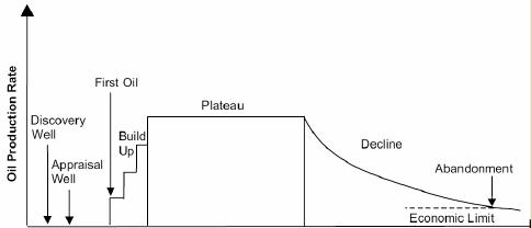
Figure 1. Idealized production behaviour of an oil field. Source: Höök et al (2009a).
The extraction of oil from a reservoir is commonly divided into 3 production methods: primary, secondary and tertiary recovery. Several factors control the production flows in most oil fields. A basic understanding of these is necessary for better understanding of decline and depletion behavior. Physically, oil recovery is about fluid flows through the porous material that make up the oil field. Fluid movements in a reservoir depend on the following factors that are explained more comprehensively by Satter et al. (2008):
- Depletion (leading to a decrease in reservoir pressure)
- Compressibility of the rock/fluid system
- Dissolution of the gas phase into the liquid
- Formation dip
- Capillary rise through microscopic pores
- Additional energy provided from the underlying aquifer or the overlying gas cap
- External fluid injection
- Thermal, or other, manipulation of fluid properties
Fluid flow fundamentals
The extraction of oil is to a large extent decided by physical properties related to the geological formation of the reservoir in question and the fluid characteristics of the petroleum it contains. Variations in these characteristics cause production rates to vary from field to field. An oil reservoir carries its fluid in small microscopic pores within the rock, and the term porosity refers to the fraction of the pore volume compared to the total bulk volume. The larger the porosity, the better the rock is at storing fluids. The pores serve both as storage and as a transmission network for fluid flows. The French physicist Henry Darcy (1856) studied fluid flow through a bed of packed sand and derived an elegant expression to describe the behavior of the fluid, known as Darcy’s law (Equation 1). The expression involves important physical properties such as the ability of the porous medium (rock in case of oil reservoirs) to permit fluid flow, its permeability, and the degree of internal resistance to flow of the fluid, its viscosity. Viscous forces tend to influence reservoir flows of both produced and injected fluids in reservoirs under normal oil field conditions to a greater extent than gravity/capillary forces. This implies that fluids flow through porous media in parallel layers with few disruptions (i.e. laminar flow conditions) and the flow rate is proportional to the existing pressure gradient in the reservoir (Satter et al., 2008).
Generally horizontal flow is greater than vertical flow due to directional differences in permeability (Selley, 1998), but this must be seen as a simplification of the real conditions in an oil field. Nevertheless it is relevant because it expresses the physical limits to the possible production rate, or defines a “best case-scenario” of production from a homogenous reservoir where the pressure gradient is the sole drive mechanism.
Darcy’s Law states that a fluid with high viscosity will have a low flow rate; that if the rock permeability is high there will be a high flow rate; and that there must be a pressure gradient in order to have any fluid flow.
Primary recovery uses naturally occurring energy, such as buoyancy (Archimedes principle) and reservoir pressure, to drive oil flows to the surface. Oil is simply allowed to flow under its own pressure, unless fluids are injected into the reservoir. However, the pressure gradient drops as oil is extracted and this will limit the rate of production according to Darcy´s law (Abrams and Wiener, 2010). This results in a depletion-driven decline in the rate of production as depletion of the reservoir reduces pressure and hence fluid flows. Reservoir and fluid properties can greatly influence the outcome and lead to significant differences in the percentage of ‘oil in place’ that is recovered (i.e. recovery factor). Typically, about 10–30% of the oil in place can be extracted during primary recovery (Kjärstad and Johnsson, 2009).
Secondary recovery focuses on artificial pressure maintenance (APM), where injection of fluids maintains reservoir pressure. In most oil fields, especially those of significant size, secondary recovery accounts for the largest proportion of total recovery (Amit, 1986; Hyne, 2001). The most common method for maintaining pressure during secondary recovery is water flooding, where water is injected to maintain reservoir pressure. When this works well the water forms a water bank that moves through the pores and presses the oil towards the producing wells. The injection of water is generally intended to give a fairly constant pressure at the entry to a well pipe (i.e. downhole pressure), but eventually injected fluids will break through and mix with the oil. Conservation of mass (i.e. material balance) in oil reservoirs requires that the extracted volume of fluid is relatively constant throughout the lifetime (Satter et al., 2008), but the water share (or ‘water cut’) will increase with time. As oil is extracted from the reservoir, an increased water cut will cause a decline of the oil production flow despite high reservoir pressure.
Water-flooding presents numerous engineering challenges that vary with the rock and fluid properties, reservoir heterogeneities and the physical differences between the oil in place and the injected water (Satter et al., 2008). One example is when the oil is much more viscous than the injected water causing so called “fingering”, where water moves in thin irregular ‘fingers’ instead of as a unified front. This bypasses significant volumes of recoverable oil and can cause premature breakthrough of water into production wells.
The properties of the oil compared to water are so important for oil extraction that the American Petroleum Institute has constructed a measure of the density of the oil compared to water, defined as API gravity = (141.5/specific gravity at 60 degrees Fahrenheit) – 131.5.
API > 10° the oil is lighter and floats on fresh water, while if API < 10° it is denser and sinks. Water flooding is possible when the oil API > 25° and the viscosity is rather low (< 30 centipoise), and works best in homogenous reservoirs. Consequently, secondary recovery is not always effective, even though a majority of the world’s oil producing fields attempt secondary recovery.
Primary and secondary recovery combined can usually extract 30–50% of the oil in place and nearly all reservoirs that can benefit from APM are using it (Kjärstad and Johnsson, 2009).
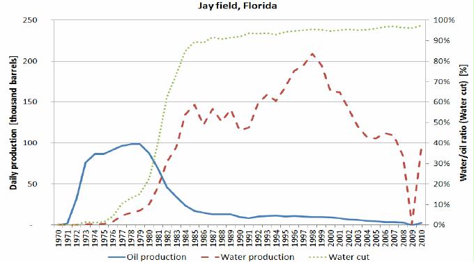
Figure 2. Production of oil and water for the giant Jay field in Florida, USA. The water cut reached over 90% of total produced fluids in the mid-1980s and is now at 97%. In 2010, the field produced 2,500 barrels of oil and 94,000 barrels of water per day. Data source: Florida Department of Environmental Protection (2012)
Tertiary recovery or enhanced oil recovery (EOR), involves more complex ways of influencing rock and fluid properties. The feasibility of EOR, together with the appropriate approach to EOR, will vary with the fluid properties and geological characteristics of the reservoir. According to Darcy’s Law, the ability of oil to move in a reservoir can be increased by decreasing its viscosity. This leads to four main approaches to EOR, namely thermal, chemical, miscible and microbial methods.
- Thermal methods are the most commonly used approach and make up nearly half of all worldwide EOR projects. Thermal EOR involves changing oil viscosity by thermal means, such as steam flooding, hot-water flooding or in-situ combustion, where the bottom of the reservoir is ignited and heat is generated by burning a part of the oil in place.
- Miscible methods account for about 41% of worldwide EOR projects and focus on injection of a gas or solvent that is miscible with the oil, resulting in improved recovery. Miscibility increases the mobility of the oil, but also greatly adds to the complexity of the process. Carbon dioxide injection is widely applicable to many reservoirs at lower miscibility pressures than other methods. Part of the carbon dioxide is soluble in oils and swells the net volume and reduces viscosity. As miscibility develops, both CO2 and oil can flow together because of the low interfacial tension. If available, light hydrocarbons (primarily natural gas) can also be injected to generate miscibility, decrease the viscosity of the oil and increase oil volume via swelling. Nitrogen, or even flue gas, is an alternative in high permeability reservoirs containing light oil (Bath, 1989). These gases are usually rather inexpensive, but inferior to CO2 or hydrocarbons from an oil recovery perspective (Satter et al., 2008). Nitrogen has poor solubility in oil and requires much higher pressures to develop miscibility.
- Chemical flooding uses the injection of polymer, surfactants, and caustic alkaline or other chemicals. At present, it makes up about 11% of global EOR projects. This technique requires conditions favorable for water-flooding as it is a modification of water-flooding. Polymers can be used to augment water-flooding by changing water viscosity and mobility. More oil will be produced in the early life of the water flood and this is the primary economic advantage, as ultimate recovery is generally the same for as for conventional water-flooding. Surfactants recover additional oil by enhancing mobility and solubility of oil and emulsification of oil and water. Caustic alkaline injection involves the injection of sodium compounds that can react with organic petroleum acids in certain oils to create surfactants in situ. Injected chemicals can also react with reservoir rocks to change wettability and thereby improve recovery. Sheng (2011) reviewed these methods.
- The final form of EOR uses microbes to improve oil recovery. It is a rarely used approach and only makes up 0.6% of worldwide EOR projects . Injected microbes can generate gas within the reservoir, thus increasing reservoir pressure and reducing oil viscosity. Alternatively microbes can generate bio-surfactants that can reduce interfacial tension and improve recovery by favourably changing wettability (Adasani and Bai, 2011).
Under favorable conditions, the combination of primary and secondary recovery can extract between one third and one half of the original oil in place. The average recovery from petroleum reservoirs around the world is estimated to be approximately 35%. If a large part of the oil remains after both primary and secondary recovery, operators may implement a suitable EOR technique. However, only a small percentage of all oil fields are using EOR due to high costs and technology requirements.
Since 1959, only 652 EOR projects have been pursued and enhanced production corresponded to ~1.8 Mb/d in 2010, or 1.5% of total global production.
Defining decline and depletion rates
The concept of depletion is intuitive as it is something of which we all have every-day experience. For example, if we have a fixed amount of beer in a bottle, and drink some of it, the beer in the bottle is unavoidably depleted. Any resource that is extracted faster than it is produced is subject to depletion – which means that depletion is not restricted to nonrenewable resources. For example, wood can be considered renewable, but if deforestation is faster than reproduction the resource is depleted within the time-span considered. A resource can only be considered as renewable if the rate of extraction is less than or equal to the rate of increment of the resource.
Fossil fuels are only reproduced on geological timescales, making depletion of these resources irreversible. While the concept of depletion is the same for all resources, there may also be limits on the rate of depletion of a resource. This is an important consideration for oil resources, where the rate of depletion is constrained by geological conditions and the physical laws of fluid flow in porous media, together with economic and technological factors.
Fundamental definitions for oil depletion
A fundamental parameter concerning oil production is the size of recoverable resources remaining for exploitation. Multiple classification schemes for resources and reserves make it difficult to compare and combine data from different sources.
Revisions to URR estimates may occur at any time as a consequence of changing market conditions, increased geological knowledge, and improved technology and so on. This makes URR a time varying quantity, although it is not as fluctuating as other reserve estimates. URR may also be expressed as the remaining recoverable resource plus cumulative production at an arbitrary point in time. Depletion levels can vary from 0 to 1 (i.e. 0–100%) and indicate what proportion of the estimated URR remains. Returning to the beer bottle analogy, we note that a half-full bottle would have a depletion level of 50%.
Depletion rates
Conceptually, the depletion rate is the ratio of annual production to some estimate of recoverable resources, where the latter can be defined as 1P or 2P reserves, remaining recoverable resources or the URR.
A lack of standardized use has resulted in several studies using depletion rates based on very different definitions of recoverable resources and this has added to the confusion surrounding the concept.
In practice, a depletion rate can refer to two possible things.
- It can relate to the rate of change of the depletion level at time t.
- Or it could also refer to the rate at which remaining recoverable resources are being produced.
Decline rates
The rate of decline, Y, is equal to the difference in the rate of production from one period to the next (change in production rate/production rate) and is commonly expressed on an annual or monthly basis. Changes can be both positive and negative, but are generally negative after a field has passed its peak of production.
A disadvantage of decline rate studies is that they do not necessarily relate to the physical factors driving oil depletion (decreasing reservoir pressure, increasing water cut, etc.). Observed decline may also arise from non-physical factors such as underinvestment, politics, production quotas, damage or sabotage. In essence, decline rates easily provide ambiguous signals for unwary analysts. Usually, decline of production is the result of complex interactions between reservoir physics, technology, economics and decision-making. Many factors influence production rates and one must be careful in extrapolating decline into the future. Decline and disruption caused by socioeconomic events are often termed ‘aboveground’ constraints, and may be resolved if proper measures are taken. On the other hand, depletion-driven decline is the result of intrinsic, below- ground physical constraints and is difficult to alleviate.
Empirical study
This study relies on the Uppsala giant oil field database. The database was initiated by Robelius (2007) and later updated by Höök et al. (2009a, b). It contains ~350 giant oil fields worldwide accounting for an URR of over 1100 Gb. For the purpose of this study, complementary data on hundreds of smaller oil fields all over the world have been combined with the giant oil field data. From this combined database, some 880 individual oilfields were selected. They were chosen to reflect the wide array of field sizes, production strategies, and socioeconomic conditions seen over the globe. The size distribution is given in Table 2, and in general an equal number of fields in each size category have been chosen. However, due to the limited number of post-peak fields larger than 1 billion barrels (Gb), this size category contains fewer fields (N=130) than the other categories (N=150). However, this difference is assumed to be negligible when identifying the general patterns of behavior.
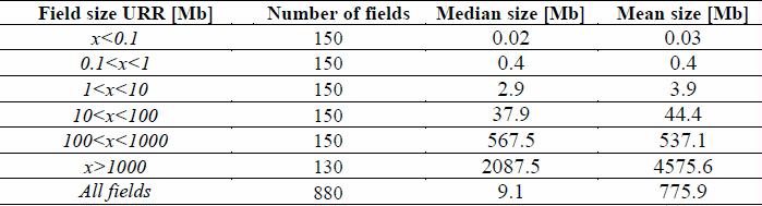
Table 2. Descriptive statistics of the sample of fields studied. The distribution is highly
skewed with most resources concentrated in relatively few giant fields.
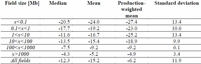
Table 3. Observed annual decline rates in percent sorted by field size.
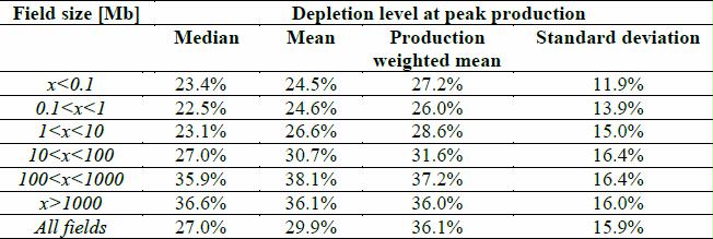
Table 5. Estimated depletion levels at peak production sorted by field size.

Table 6. Estimated depletion rates of ultimately recoverable resources at onset of decline, sorted by field size.
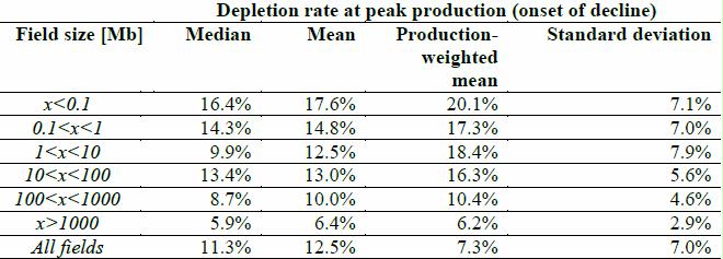
Table 7. Estimated depletion rates of remaining recoverable resources sorted by field size.
Data considerations
To assess depletion and decline rate behavior, data for individual fields is essential. Some data on production and recoverable resources is available in the public domain or can be obtained from companies (IHS, Rystad Energy, etc.), agencies or governments. Some regions, such as the North Sea, provide excellent openly accessible data while others, such as OPEC, are characterized by generally poor data access.
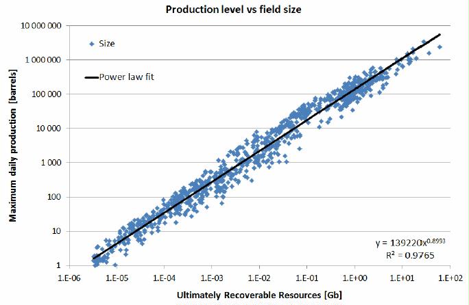
Figure 5. The relation between field size and maximum production level.
Annual or monthly production data is comparatively easy to acquire and can commonly be obtained from operators, agencies or third-party sources such as business magazines, trade journals, etc. Recoverable resources, reserve estimates, and related data are more problematic to acquire and are generally less reliable. The multiple classification schemes for resources and reserves make it difficult to compare and combine data from different sources (UKERC, 2009a).
Naturally, there are shortcomings in the available data. For example, different definitions among reporting agencies, changing classifications over time, terrorist strikes, major accidents (Piper Alpha, Deepwater Horizon, etc.), and political decisions can all influence both production trends and data quality. Fields with severely disturbed behavior or otherwise dubious properties were, as far as possible, omitted from this analysis. Some fields exhibit a clear peak, commonly quite early in the field’s life, followed a decline phase. Other fields can have long plateau phases, possibly ranging for decades, which are followed by the onset of decline.
This study focuses on fields that have “peaked” and left the plateau stage. Consequently, fields that are in the build-up phase or haven’t reached the onset of decline are excluded from the study. For fields with a plateau, “peaking” was defined as the point where production is judged to clearly leave a 4% fluctuation band around the plateau level, as earlier used by Höök et al. (2009b). The data show a strong correlation (R2 = 0.98) between estimated URR and peak/plateau production levels (a power fit indicates a strong correlation valid over several magnitudes as seen in figure 5). This is hardly surprising, since high daily production levels are generally only possible in fields with significant URR.
For some fields, official estimates of URR or equivalent were available. For others, the URR was estimated by adding cumulative production to recent (no older than 2005) industry estimates of 2P (proven+probable) reserves. Bentley et al. (2007) discuss industry 2P data in more detail and suggest that they provide a median estimate of remaining recoverable resources (i.e. there is a 50% probability that recoverable resources are higher or lower). Thus it is equally likely that cumulative production over the remaining life-time of the field will be greater or lower than the 2P figure. However, reserve estimates tend to increase over time, a phenomenon known as reserve growth (Sorrell et al., 2012). Factors such as increased investment, technology and knowledge are also acknowledged and known to increase reserves over time, making it probable that URR estimates based upon current 2P reserves will underestimate the actual field size, and the fact of reserves growth must also be acknowledged even in 2P data. For the remainder where no 2P data or official URR estimates were available, more traditional curve-fitting methods were used to estimate the URR.
In our aggregated dataset, the URR of some fields are surely overestimated, while others may be underestimated. We assume here that these effects cancel each other out when combined. For the sake of simplicity we assume here that a field’s URR remains fixed over time. Changed URR values will not affect decline rates of any of the fields used in this study, and neither will it affect the peak production points. However, increases in the estimated URR reduce the estimated depletion level and depletion rate.
Decline rates seen in real fields can vary significantly. In this dataset, annual decline rates ranged from less than 1% to more than 70%, although the range decreases with increasing field size (Figure 6). The average decline rates for the entire data set can be derived, although such a figure can be misleading due to the underlying size dependence. Closer analysis shows major differences among decline rates and implies that decline rates of small fields may differ significantly from those of large fields (Table 3).
Giant fields of over 1 Gb have by far the lowest decline rates and there is a clear trend towards more rapid decline with decreasing field size (Table 3). Production-weighted (PW) average values also show that fields with high production levels tend to decline somewhat faster than the arithmetic average for small fields (<0.1 Gb), while the opposite was true for semi-giant and giant oil fields. Partly this can be explained by a large share of OPEC control among the larger fields and the fact that OPEC producers tend to aim for long and stable production profiles rather than rapid return on investment. Secondly, these patterns can arise from the economically rational behavior of a price- taking producer who maximizes profit subject to technical and physical constraints (Jakobsson et al., 2012).
Table 3. Observed annual decline rates in percent sorted by field size.
Earlier studies have also shown that technological development such as EOR can result in more rapid declines. Gowdy and Julia (2007) initially highlighted this problem for two North Sea giant fields. Later, Höök et al. (2009a, b) elaborated on this and found a general tendency towards higher decline rates for giant fields as new technology and modern production strategies allowed the extension of plateau production at the expense of higher subsequent decline rates.
Table 4 compares the results of three studies that provide estimates of average decline rates from a globally representative sample of post-peak giant fields. Despite differences in data sets, definitions and weighting methods, the results are in broad agreement that the decline in the existing production is between 4–8% annually (Höök et al., 2009b). Expressed in production capacity, this means that roughly a new North Sea (~5 Mb/d) has to come on stream every year just to keep the present output constant (Fantazzini et al., 2011). This implies that nearly 5 new Saudi-Arabias would be needed by 2030 just to offset the decline in existing production (Aleklett et al., 2010).
Höök et al. (2009b) provides additional data on the time evolution of giant oil field decline rates and finds the average decline rate has increased by around 0.15% per year since mid-1960s – a trend that is expected to continue. From Table 3, it can be also seen that decline rates are higher for smaller fields and as future production becomes more reliant on non-giant fields it is reasonable that average decline in existing production will increase. The Increasing decline rate is seldom discussed – even though it can lead to additional capacity requirements of as much as 7 Mb/d by 2030 (Aleklett et al., 2010).
Figure 6. Scatter plot of observed decline rates seen the data set. Significant differences occur, but generally decrease with increasing field size.
Table 4. Average decline rates for post-peak giant fields found by recent studies. Source: Höök et al. (2009b) Parameter Höök et al. IEA CERA Average decline
Depletion level behavior
Earlier studies have shown that it is common for giant oil fields to reach the onset of decline when less than half of the URR has been produced (Höök et al., 2009a). In this study, this analysis is expanded to include smaller fields. Figure 7 provides a scatter plot of the estimated depletion level at the onset of decline, while Figure 8 provides a corresponding frequency histogram.
A significant spread can be seen among the fields studied with some reaching an estimated depletion level of over 80% before the onset of decline, while others peak at depletion levels as low as 10%. However, there is a clear trend towards higher depletion levels at peak with increasing field size (Table 5). Some of the fields with the highest depletion levels at peak, especially in the >100 Mb size category, are old American fields that were extensively redeveloped around the 1980s when new technology/investments allowed larger fractions of the oil- in-place to be recovered. Production-weighted figures indicate that fields with high annual production rates are usually developed in such a way that the depletion level is relatively high at the onset of decline.
Interestingly, there is virtually no correlation (linear correlation coefficient = -0.07) between the estimated depletion levels at peak and the subsequent decline rates in oil fields. This indicates that depletion levels have restricted relevance for analyzing production flows.
It should also be noted that any future reserve growth in the studied fields will reduce the estimated depletion levels. If a significant portion of the URR figures used in this study are underestimates, the depletion levels derived here will be overestimates. If so, this would reinforce the conclusion that most fields begin to decline well before half of their URR is produced.
Figure 7. Scatter plot of estimated depletion levels at peak production (onset of decline).
The theory described above predicts that maximum depletion rates should occur when the onset of decline is reached. This may also be referred to as the depletion rate at peak and effectively marks the point where depletion-driven decline begins to dominate over other variables and leads to the onset of production decline. Estimated annual depletion rates of URR at the onset of decline are plotted in Figure 9. A few small fields reach depletion rates of 30% or more before peaking, but most have significantly lower depletion rates at peak production. The histogram (Figure 10) shows a skewed distribution with the largest number of fields having values of 10% or less, leading to an overall mean of 10.3% and a production-weighted mean of 4.9%. The figure also demonstrates a clear trend towards lower depletion rates at peak with increasing field size (Table 6).
The general behavior is similar for depletion rates of remaining recoverable resources (RRR) as seen in Figure 11. The distribution histogram (Figure 12) shows a skewed structure with only a small number of fields capable of depleting more than 20% of the remaining recoverable resources per year at peak production. Depletion rate differences diminish with increasing field size, indicating a narrowing interval of possible depletion rates. Höök et al. (2009a) expanded on this correlation by comparing onshore, offshore, OPEC, and non-OPEC giant oil fields.
High depletion rates are only common in small oil fields, and are increasingly exceptional with increasing field size. As noted earlier, an oil-producing region consists of a sum of individual oil fields, with their individual peak points distributed in time. From the theory described in Section 3.4, it follows that the regional depletion rate must be somewhere between the minimum and maximum depletion rates of its components. Maximum depletion rates can only be reached if all fields peak simultaneously, which is extremely unlikely. According to our analysis of field data, regional depletion rates are likely to be constrained to less than 20% if they are assumed to follow patterns seen in history. Given the dominance of larger fields in total regional production, the regional depletion rates are even lower in reality. Aleklett et al. (2010) estimates that the typical regional depletion rates of remaining recoverable resources are of the order of 2–5%, and argue that projections of future global oil production by the IEA (2008) are based upon unrealistic assumptions about depletion rates that are not explicitly discussed. Miller (2011) agrees with the findings of Aleklett et al. (2010) and notes the persistent optimism of the IEA projections.
Depletion rates can be directly calculated from production data and URR estimates during both the build-up and plateau stages in an oil field’s life, even before the field has peaked.
In contrast, decline rates can only be estimated after the onset of decline.
However, the strong correlation between the concepts makes it possible to use depletion rates to estimate future average decline rates reasonably well. This has already been used to forecast future production profiles for fields that have yet to reach the onset of decline (Höök et al., 2010b). When combined with reliable URR estimates, depletion rate analysis offers a simple tool for making educated estimates of future production decline rates.
Decline and depletion rates are important to understand and give significant depth to the peak oil debate. However, it is essential to understand that these two concepts are fundamentally different. Decline rates can be measured directly from production data, while depletion rates depend upon estimates of recoverable resources. Changes in recoverability will affect depletion levels and depletion rates, while decline rates are unaffected. Different data sources and resource estimates done at different times are likely to give diverging results.
Oil field size is a key variable, with generally high values for most parameters in small fields and comparatively low values for larger fields. The data shows clearly that most fields tend to peak with much less than half of their ultimately recoverable resources produced, typically around 30% (Table 5).
Peak production generally appears well before the glass is half empty.
Depletion levels of giant oilfields are a noteworthy detail, since giant fields tend to reach the onset of decline with higher depletion levels than small fields. This could be explained by the way most giant fields are developed, as they usually start production at far lower depletion rates than smaller fields due to requirements related to production equipment, pipelines, etc. As a result, giant fields can maintain production plateau by continually drilling into new parts of the reservoir to supplement declining production from older sections and this can probably lead to comparatively higher depletion levels at peak. However, this could also be an effect of underestimated URR and might possibly change if significant future reserve growth occurs.
The theoretical framework summarized here is well supported by the empirical evidence. The existence of maximum depletion rates prior to the onset of production decline is of particular importance. Furthermore, the strong correlation between depletion rates at peak and subsequent decline rates can be used in supply forecasting and for estimating future decline rates before the plateau phase ends. Depletion rate analysis has been around for some time, but the underlying methodology has never been clearly presented.
Much confusion surrounds the concept of depletion rates, even though it is relatively simple idea once properly understood. Maugeri (2012) is a recent example of how terminology is mixed up and how exceptionally low decline rates are used without any solid justification.
Another example is how the EIA used a depletion rate model in a flawed way to reach misleading conclusions (Jakobsson et al., 2009). Similarly, the IEA’s influential projections of global oil supply are based upon highly unrealistic assumptions about the depletion rates of various categories of resources (UKERC, 2009a; Aleklett et al., 2010; Miller, 2011). Once more realistic assumptions are made; the future supply outlook looks much bleaker.
References
Abrams, D.M., Wiener, R.J., 2010. A model of peak production in oil fields. American Journal of Physics, 78(1), 24–27. DOI: http://dx.doi.org/10.1119/1.3247984
Adasani, A., Bai, B., 2011. Analysis of EOR projects and updated screening criteria. Journal of Petroleum Science and Engineering, 79(1–2), 10–24. DOI: http://dx.doi.org/10.1016/j.petrol.2011.07.005
Aleklett, K., Höök, M., Jakobsson, K., Lardelli, M., Snowden, S., Söderbergh, B., 2010. The Peak of the Oil Age – analyzing the world oil production Reference Scenario in World Energy Outlook 2008. Energy Policy, 38(3), 1398-1414. DOI: http://dx.doi.org/10.1016/j.enpol.2009.11.021
Amit, R., 1986. Petroleum reservoir exploitation: switching from primary to secondary recovery. Operations research, 34(4), 534–549. DOI: http://dx.doi.org/10.1287/opre.34.4.534
Arps, J.J., 1945. Analysis of decline curves. Transactions of the American Institute of Mining, Metallurgical and Petroleum Engineers, 160, 228–247.
Arps, J.J., 1956. Estimation of primary oil reserves. Transactions of the American Institute of Mining, Metallurgical and Petroleum
Engineers, 207, 182–191.
Bath, P.G.H., 1989. Status report on miscible/immiscible gas flooding. Journal of Petroleum Science and Engineering, 2(2–3), 103–117. DOI: http://dx.doi.org/10.1016/0920-4105(89)90057-0
Bentley, R.W., Mannan, S.A., Wheeler, S.J., 2007. Assessing the date of the global oil peak: the need to use 2P reserves. Energy Policy, 35(12), 6364–6382. DOI: http://dx.doi.org/10.1016/j.enpol.2007.08.001
Campbell, C., 1992. The depletion of oil. Marine and Petroleum Geology, 9(6), 666–671.
Campbell, C., 1996. The status of world oil depletion at the end of 1995. Energy Exploration and Exploitation, 14(1), 63–81.
Campbell, C., 2006. The Rimini Protocol an oil depletion protocol: Heading off economic chaos and political conflict during the second half of the age of oil. Energy Policy, 34(12), 1319–1325. DOI: http://dx.doi.org/10.1016/j.enpol.2006.02.005
Campbell, C., Heapes, S., 2008. An atlas of oil and gas depletion. Jeremy Mills Publishing, Huddersfield, 396 p.
Chang, C.P., Lin, Z.S., 1999. Stochastic analysis of production decline data for production prediction and reserves estimation. Journal of Petroleum Science and Engineering, 23(3-4), 149–160. DOI: http://dx.doi.org/10.1016/S0920-4105(99)00013-3
Darcy, H., 1856. Les Fontaines publiques de la Ville de Dijon. Vitor Dalmont, Paris, 666 p.
van Everdingen, A.F., Hurst, W., 1949. The application of the Laplace transformation to flow problems in reservoirs. Journal of Petroleum Technology, 1(12), 305–324. DOI: http://dx.doi.org/10.2118/949305-G
Fantazzini, D., Höök, M., Angelantoni, A., 2011. Global oil risks in the early 21st Century. Energy Policy, 39(12), 7865–7873. DOI: http://dx.doi.org/10.1016/j.enpol.2011.09.035
Florida Department of Environmental Protection, 2012. Oil, gas and water production data compiled by field and region.
Flower, A.R., 1978. World oil production. Scientific American, 238(3), 42–49.
Gowdy, J., Juliá, R., 2007. Technology and petroleum exhaustion: Evidence from two mega-oil fields. Energy, 32(8), 1448–1454. DOI: http://dx.doi.org/10.1016/j.energy.2006.10.019
Hurst, R., 1934. Unsteady flow of fluids in oil reservoirs, Journal of Applied Physics, 5(20), 20–30.
Hyne, N.J., 2001. Nontechnical guide to petroleum geology, exploration and production. Second edition, Pennwell Corporation, 2001, 575 p.
Höök, M., Söderbergh, B., Jakobsson, K., Aleklett, K., 2009a. The evolution of giant oil field production behaviour. Natural Resources Research, 18(1), 39–56. DOI: http://dx.doi.org/10.1007/s11053-009-9087-z
Höök, M., Hirsch, R., Aleklett, K., 2009b. Giant oil field decline rates and their influence on world oil production. Energy Policy, 37(6), 2262–2272. DOI: http://dx.doi.org/10.1016/j.enpol.2009.02.020
Höök, M., Söderbergh, B., Aleklett, K., 2009c. Future Danish oil and gas export. Energy, 34(11), 1826–1834. DOI: http://dx.doi.org/10.1016/j.energy.2009.07.028
Höök, M., Bardi, U., Feng, L., Pang, X., 2010a. Development of oil formation theories and their importance for peak oil. Marine and Petroleum Geology, 27(9), 1995–2004. DOI: http://dx.doi.org/10.1016/j.marpetgeo.2010.06.005
Höök, M., Tang, X., Pang, X., Aleklett, K., 2010b. Development journey and outlook of Chinese giant oil fields. Petroleum Exploration and Development, 37(2), 237–249. DOI: http://dx.doi.org/10.1016/S1876-3804(10)60030-4
IEA, 2008. World Energy Outlook 2008. Available from http://www.worldenergyoutlook.org/publications/2008-1994/
IEA, 2011. Key energy statistics 2011. See also: http://www.iea.org
Jackson, P. and Smith, 2013. Exploring the undulating plateau: the future of global oil supply. Philosophical Transactions of the Royal
Society Series A, this volume.
Jakobsson, K., Söderbergh, B., Höök, M., Aleklett, K., 2009. How reasonable are oil production scenarios from public agencies? EnergyPolicy, 37(11), 4809–4818. DOI: http://dx.doi.org/10.1016/j.enpol.2009.06.042
Jakobsson, K., Bentley, R., Söderbergh, B., Aleklett, K., 2012. The end of cheap oil: Bottom-up economic and geologic modeling of aggregate oil production curves. Energy Policy, 41, 860–870. DOI: http://dx.doi.org/10.1016/j.enpol.2011.11.073
Khanamiri, H.H., 2010. A non-iterative method of decline curve analysis. Journal of Petroleum Science and Engineering, 73(1-2), 59–66. DOI: http://dx.doi.org/10.1016/j.petrol.2010.05.007
Kjärstad, J., Johnsson, F., 2009. Resources and future supply of oil. Energy Policy, 37(2), 441–464.
DOI: http://dx.doi.org/10.1016/j.enpol.2008.09.056
Kovscek, A.R., 2012. Emerging challenges and potential futures for thermally enhanced oil recovery. Journal of Petroleum Science and Engineering, in press. DOI: http://dx.doi.org/10.1016/j.petrol.2012.08.004
Maugeri, L., 2012. Oil: the next revolution. The unprecedented upsurge of oil production capacity and what it means for the world. Report from the Belfer Center for Science and International Affairs. June 2012. Available from: http://belfercenter.ksg.harvard.edu/files/Oil-%20The%20Next%20Revolution.pdf
Miller, R., 2011. Future oil supply: The changing stance of the International Energy Agency. Energy Policy, 39(3), 1569–1574. DOI: http://dx.doi.org/10.1016/j.enpol.2010.12.032
Muggeridge, A., Cockin, A., Webb, K., Frampton, H., Collins, I., Moulds, T., Duncan, E, 2013. Recovery rates, enhanced oil recovery and technological limits. Philosophical Transactions of the Royal Society Series A, this volume.
Neuman, S.P., 1977. Theoretical derivation of Darcy’s law. Acta Mechanica, 25(3-4), 153–170.
DOI: http://dx.doi.org/10.1007/BF01376989
Robelius, F., 2007. Giant oil fields – the highway to oil: giant oil fields and their importance for future oil production. Doctoral thesis from Uppsala University, 156 p. See also: http://publications.uu.se/abstract.xsql?dbid=7625
Satter, A., Iqbal, G.M., Buchwalter, J.L., 2008. Practical enhanced reservoir engineering. Pennwell Books, 688 p.
Saudi-Aramco, 2004. Fifty-year crude oil supply scenarios: Saudi-Aramco’s perspective. Presentation given by M.M Abdul Baqi and N. G.
Saleri at CSIS, Washington, D.C. February 24, 2004.
Selley, R., 1998. Elements of petroleum geology. Academic Press, USA, 470 p.
Sheng, J.J., 2011. Modern chemical enhanced oil recovery – theory and practice. Gulf Professional Publishing. ISBN: 978-1-85617-745-0. 648 p.
Sorrell, S., Speirs, J., Bentley, R., Miller, R., Thompson, E., 2012. Shaping the global oil peak: A review of the evidence on field sizes, reserve growth, decline rates and depletion rates. Energy, 37(1), 709–724. DOI: http://dx.doi.org/10.1016/j.energy.2011.10.010
UKERC, 2009a. Global oil depletion – an assessment of the evidence for a near-term peak in global oil production. Report by the UK Energy Research Centre, August 2009. Available from: http://www.ukerc.ac.uk/support/Global%20Oil%20Depletion
UKERC, 2009b. Nature and importance of reserve growth. Technical report 3, July 2009. Available
from: http://www.ukerc.ac.uk/support/Global%20Oil%20Depletion