
NREL. 2008. Determining the Capacity Value of Wind: An Updated Survey of Methods and Implementation. National Renewable Energy Laboratory.
Electric systems must have sufficient reserves so that resources are adequate to meet customer demand. Because electricity demand cannot be known in advance with certainty, and because generation can experience mechanical or electrical failures which take it out of service (i.e., experience forced outages), a planning reserve that consists of installed capacity in excess of load requirements is necessary to maintain reliability. This reserve is applied in the planning time frame (i.e., one year or more), and is a determination of system adequacy: is there sufficient installed generation to meet load obligations?
The level of wind capacity value is a matter of debate in some regions, due to the variability of wind power and its relationship with load. Utilities and other entities typically allocate some capacity value to wind power, although at a lower level than other energy technologies.
With over 18 GW of installed wind capacity in the United States as of first quarter 2008, and another 4 GW under construction, the question of wind’s capacity value (sometimes called capacity credit) is gaining more attention. System planners will need to grapple with how to determine the capacity value of wind energy. It is clear that wind’s primary value is as an energy resource, but the extent to which it contributes towards system adequacy is an important question. Effective load carrying capability (ELCC) is an often-used metric to assess capacity credit, not only for wind plants, but for any power plant. A typical power plant has a relatively low forced outage rate, which implies a high availability rate. This translates into an ELCC value that is typically a large percentage of the conventional plant rated capacity.
Because wind generators only generate electricity when the wind is blowing, wind’s availability rate (the rate that power and energy can actually be provided) is a function of the wind speed throughout the year. Therefore, the effective forced outage rate for wind generators may be much higher, from 50% to 80%, when recognizing the variable availability of wind. In addition, wind’s value to the electric system may also vary. The output from some wind generators may have a high correlation with load and thereby can be seen as supplying capacity when it is most needed. In this situation, a wind generating plant should have a relatively high capacity credit. The output from other wind generating plants may not be as highly correlate d with system load, and therefore would have a lower value to the electric system a nd should receive a lower capacity credit. The correlation of wind generation with system load, along with th e wind generator’s outage rate, is the primary determinants of wind capacity credit.
With modern interconnected power systems, the LOLP does not necessarily measure the probability that load will be shed because of insufficient generation. The LOLP metric measures the risk that generation cannot meet the peak demand unless capacity is imported. When performing a reliability analysis it is necessary to sel ect a risk target. This is often chosen to be a LOLE of 1 day per 10 years. This roughly corresponds to a 0.9997 probability that generation will be sufficient to cover load without unexpected imports.
ELCC is driven by the timing of high LOLP hours. Figure 3 shows a typical LOLP duration curve. A generator that contributes a signifi cant level of capacity during the top 200 hours will have a higher capacity value (ELCC) than a unit that delivers the same capacity during hours 600 – 800 instead. Generators that reduce LOLP the most will make the highest contribution to system adequacy and reliability, and will therefore have a higher ELCC. If a plant were unable to generate any power during the approximately 80 0 hours shown in the graph, its capacity value would be very close to zero.
To calculate ELCC, a database is required that contains hourly load requirements and generator characteristics. For conventional generators, ra ted capacity, forced outage rates, and specific maintenance schedules are the primary requirement s. For a variable resource such as wind, at least one year of hourly power output is required, but more data is always better.
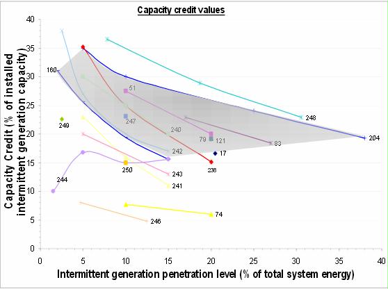
My comment: As you can see blow, the higher the penetration level, the less capacity credit, because the more you depend on wind, the less likely it is to be there when you need it the most at peak periods:
House of Lords. 2007-2008. The Economics of Renewable Energy. House of Lords Select Committee on Economic Affairs 4th Report, Great Britain.
Peak demand and capacity credit
A cost due to intermittency comes from the need to have enough capacity available to meet peak demand. No power station is guaranteed to be available at peak demand. So industry holds extra capacity over and above the expected peak demand to cope with stations that turn out not be available when most needed, or higher than expected demand. As a rule of thumb, a 20% margin of extra capacity has been sufficient to keep the risk of a power cut due to insufficient generation at a very low level.
A fossil-fueled station has around a 5% chance of not being available to generate at the time of the system peak because of breakdowns or essential maintenance. One plant’s breakdown is rarely correlated with another. Nuclear plants have a similar risk.
But for renewables it is very different. At peak demand not only are the chances of a wind farm not being fully available much higher but it is very likely that, if so, nearby wind farms will also be at least partially unavailable because it is not windy in the area. This correlation will fall for distant wind farms—for example, the wind could well blow in Scotland when conditions in Cornwall are calm. But within the UK, the correlation does not fall to zero.
As a result, the proportion of renewable generation which can be relied on at peak demand is much lower than for fossil fuel plants and more complicated to calculate. We received several estimates of how far wind capacity could be counted on to contribute to meet peak demand—its “capacity credit”. BERR uses a range of between 10% and 20% of wind stations’ capacity, so that 25 GW of wind plant could displace between 2.5 and 5 GW of conventional plant. E.ON suggest that the capacity credit of wind power in the UK should be only 8%.
As wind generation increases, its capacity credit will tend to fall because low winds over part of the country can affect many wind turbines simultaneously. Extra, offsetting conventional plant is needed. The Renewable Energy Foundation’s rule of thumb is to treat the square root of the wind capacity in GW as if it were conventional capacity. On that basis, for example, 25 GW of installed wind generation capacity could be counted on for the same contribution to peak demand as 5 GW of conventional capacity; and it would take 36 GW of wind plant to match 6 GW of conventional plant.
It is clear that much conventional capacity will be required to support renewable generators coming on stream in the period up to 2020, during which many of Britain’s coal and nuclear power plants are scheduled to close. To replace them, the Government has calculated that 20–25 GW of new power stations will be needed by 2020—about a quarter of today’s 76 GW of electricity capacity. But that calculation assumes replacement on a like-for-like basis and does not take account of the target for renewables. If 30 GW of additional renewable capacity were required to meet the EU’s 2020 target for the UK (and its capacity credit was less than 6 GW), a further 14–19 GW of new fossil fuel and nuclear capacity will still be needed to replace closing plants and meet new demand. The total new installed electricity generating capacity required by 2020 would thus be roughly double the level needed if renewable generation were not expanded. [20-25 GW new power = 30 GW of wind to get 6 GW of reliable capacity plus 14-19 GW fossil / nuclear to back up wind when it’s not blowing = 44-49 GW total power]
The intermittent nature of wind turbines and some other renewable generators means they can replace only a little of the capacity of fossil fuel and nuclear power plants, if security of supply is to be maintained. Investment in renewable generation capacity will therefore largely be in addition to, rather than a replacement for, the massive investment in fossil-fuel and nuclear plant required to replace the many power stations scheduled for closure by 2020. The scale and urgency of the investment required is formidable, as is the cost.
We have a particular concern over the prospective role of wind generated and other intermittent sources of electricity in the UK, in the absence of a break-through in electricity storage technology or the integration of the UK grid with that of continental Europe. Wind generation offers the most readily available short-term enhancement in renewable electricity and its base cost is relatively cheap. The evidence presented to us implies that the full costs of wind generation (allowing for intermittency, back-up conventional plant and grid connection), although declining over time, remain significantly higher than those of conventional or nuclear generation (even before allowing for support costs and the environmental impacts of wind farms). Furthermore, the evidence suggests that the capacity credit of wind power its probable power output at the time of need) is very low; so it cannot be relied upon to meet peak demand. Thus wind generation needs to be viewed largely as additional capacity to that which will need to be provided, in any event, by more reliable means
Other documents at www.parliament.uk:
Houses of Parliament. May 2014. Intermittent Electricity Generation. Parliamentary office of science & technology PostNote number 464.
In 2013 UK wind power could produce 11 GW at maximum capacity, but only 7-25% of that figure was reliable capacity. If the proportion of generation from wind rises towards 50%, the proportional reliability of wind will fall from 17-25% (in 2013) towards 7-9%. The contribution of solar is zero because reliable capacity is measured at annual peak demand, which occurs in winter, after dark. Wind’s contribution is not zero as the wind is generally blowing somewhere in Great Britain. Fossil-fueled and nuclear had a 77-95% reliable capacity.
Motion 781: “… it is unlikely that wind farms could provide a significant part of the United Kingdom’s energy needs, given the cost of their construction, their short life span, the expense of the electricity they produce and their low generating efficiency…”
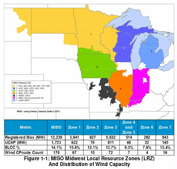
December 2013. MISO 2014 Wind Capacity Credit Report, Planning Year 2014-2015 Wind Capacity Credit.
The probabilistic measure of load not being served is known as Loss of Load Probability (LOLP) and when this probability is summed over a time frame, e.g. one year; it is known as Loss of Load Expectation (LOLE). The accepted industry standard for what has been considered a reliable system has been the “Less than 1 Day in 10 Years” criteria for LOLE. Th is measure is often expressed as 0.1 days/year, as that is often the time period (1 year) over which the LO LE index is calculated.
Effective Load Carrying Capability (ELCC) is define d as the amount of incremental load a resource, such as wind, can dependably and reliably serve, while considering the probabilistic nature of generation shortfalls and random forced outages as driving factors to load not being served. Using ELCC in the determination of capacity value for generation resources has been around for nearly half a century. In 1966, Garver demonstrated the use of loss-of-load probability mathematics in the calculation of ELCC 1 To measure the ELCC of a particular resource, the reliability effects need to be isolated for the resource in question from those of all the other sources.
This is accomplished by calculating the LOLE of two different cases: one “With” and one “Without” the resource. Inherently, the case “with” the resource should be m ore reliable and consequently have fewer days per year of expected loss of load (smaller LOLE).
Do averages have any meaning when it comes to wind?
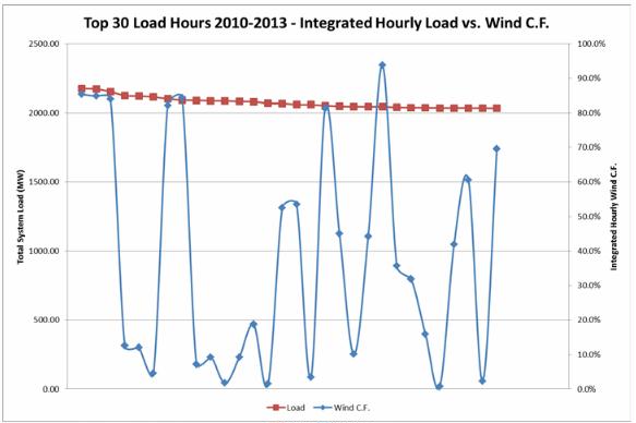
Every year a different ELCC results, but what does this figure really mean in terms of running the grid? They came up with a figure of 14%. But if you look at the MISO chart on page 12 with 72 critical peak load hours over 8 years and how much wind was blowing (the capacity), there were 39 times when it was less than 14% and 33 times when it was more. So you can’t ever rely on wind for 14% power. there were times when it was only contributing 1.6% of it’s potential, far from average capacity. You’d better have a lot of other kinds of power plants to back wind up the 54% of the time it isn’t there for you at peak load hours.
Aha! I kept looking around, and Nova Scotia Power agrees with me:
The graph below shows the 30 highest load hours over the past 4 years and the coincident available wind capacity during those hours. In this plot it can be seen that while wind generation may be present at near nameplate capacity during some high load hours, it may not be there at all in other high load hours. While the hourly capacities shown here may average to a large figure, that ELCC would not adequately represent the true system operating requirements. In fact, in 1/3 of the peak load hours shown here wind generation is at 10% or less.
This bi-modal wind generation behavior makes the inherent averaging LOLE method of calculating capacity value of wind, with matched load–wind shapes, rather optimistic. The risk of overstating capacity value of wind is designing a system with inadequate firm capacity to serve load in all peak hours.
LOLE is inherently an averaging quantity:
LOLE = Average (LOLP)/100*8784/24 Where LOLP = Loss of Load Probability As such LOLE quantity does not adequately preserve the high LOLP values impact on the system. The plot below (see slide 12) is an example of the LOLP distribution throughout a year and it illustrates why averaging of LOLP quantities into an annual LOLE quantity may not be the best method for calculating NSPI’s capacity value of wind
The cost of under-or over-estimating the capacity value of wind is asymmetrical. Over-estimating the capacity value of wind and then operating the system accordingly could result in inadequate resources to meet peak system demand. That situation has much more severe consequences than under-estimating wind resources capacity and having more than adequate resources to meet peak demands, particularly as NSPI is a winter peaking utility. There are uncertainties associated with load growth. For example, we have seen the highest system peak firm load in history in January 2014, which adds to the importance of carrying adequate planning reserve margin . The planning reserve margin can be compromised by assigning a high capacity value to wind generation in the planning process. For example, a 27% capacity value for committed wind generation of 550-600 MW means that ~150-160 MW, or 40% of the required planning reserve, may or may not be available depending on the wind generation output.
Nova Scotia used a cumulative frequency analysis to come up with a wind capacity value of 12% — GE used a different method and came up with 27% wind capacity.
Nova Scotia Power. April 2014. Capacity Value of Wind Assumptions and Planning Reserve Margin
IEA. 2013. Wind Task 25 Design and operation of power systems with large amounts of wind power. Phase two 2009–2011. International Energy Agency.
Capacity value of wind power
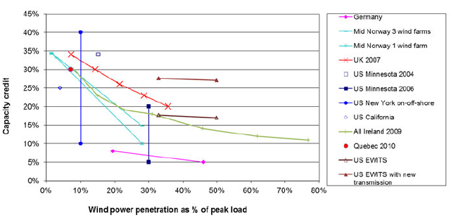
Figure 18. Capacity credit of wind power, results from ten studies, showing reduction of capacity value as penetration level increases. New York on-off-shore (blue vertical line in chart) shows the range of capacity value for wind, when calculated only for onshore sites (10%) or only offshore sites (40%).
The question of whether there is sufficient capacity at some future date is known as the power or resource adequacy question. This is related to the long-term reserve or planning reserve that power systems carry.
To answer questions such as: “Can wind substitute for other generation in the system and to what extent?” and “Is the system capable of meeting a higher (peak) demand if wind power is added to the system?” the capacity value of wind can be calculated. Capacity value is the portion of installed capacity that will provide additional load carrying capability to meet projected increases in system demand.
This contribution is typically measured in either MW or as a percentage of installed wind capacity. The term “capacity credit” may also be used. Two international task force papers (partly including Task 25 collaboration) have recommended the use of loss of load expectation (LOLE) and related methods, such as calculating the Effective Load Carrying Capability (ELCC) to calculate the capacity value of wind (Keane et al., 2011; NERC, 2011). Wind generation will have a capacity value that is often close to the average power produced by wind power (capacity factor) at low penetrations and will decline as wind penetration increases. In the results summarized in Figure 18, the range is from 40% of installed wind power capacity (in situations with low wind penetration and a high capacity factor at times of peak load), to 5% in higher wind penetrations, or if regional wind power output profiles correlate negatively with the system load profile (a low capacity factor at times of peak load). The aggregation benefits apply to capacity credit calculations – for larger geographical areas, the capacity credit will be higher. The relative wind capacity credit, as percent of installed wind capacity, is reduced at higher wind penetration, but the extent of this decrease depends on the geographical dispersion of the additional wind plants and the smoothing that results from this dispersion. This is demonstrated by comparing the cases of Mid Norway with one and three wind power plants. In essence, it means that the wind capacity credit for all installed wind in Europe or the United States is likely to be higher than that of the individual countries or regions, with the same penetration level. Indeed, this is true only when assuming that the grid is not limiting the use of the wind capacity (i.e., just as available grid capacity is a precondition for allocating capacity credit to other generation). The results presented in Figure 18 for capacity value of wind power are from the following studies: · Germany (Dena, 2005) · Ireland (AIGS, 2008) · Norway (Tande & Korpås, 2006) · Quebec (Bernier & Sennoun, 2010) · UK (Ilex Energy & Strbac, 2002) · US Minnesota (EnerNex/WindLogics, 2004 and 2006) · US New York (GE Energy, 2005) ·US California (Shiu et al., 2006) · US EWITS study (EWITS, 2010).
The US Eastern Wind Integration Study EWITS did several calculations for capacity value of wind. The study used three scenarios of 20% wind penetration and one scenario of 30% penetration. Three load and wind profile years were used for each scenario. Using the 2004 profile year, the capacity value of wind (Effective Load Carrying Capability ELCC) was 14-18% of wind rated capacity. The 2005 profile results are 14-20%, and the 2006 profile results are 16-23% (EWITS, 2010). The 30% results are 16-19% for profile years 2004-2006, respectively. When a new transmission overlay was added, the results changed significantly, ranging from 24% to 33% of wind rated capacity, depending on penetration.
The inability to integrate all wind power in the system can be seen as occasional curtailments of wind power that may be needed due to either transmission congestion or insufficient balancing or stability issues in the system. Increasing power system flexibility through increasing transmission to neighboring areas, generation flexibility, demand-side management, and optimal use of storage (e.g., pumping hydro or thermal), in combination with market aggregation and operation closer to real time, will impact the amount of wind that can be integrated cost effectively.