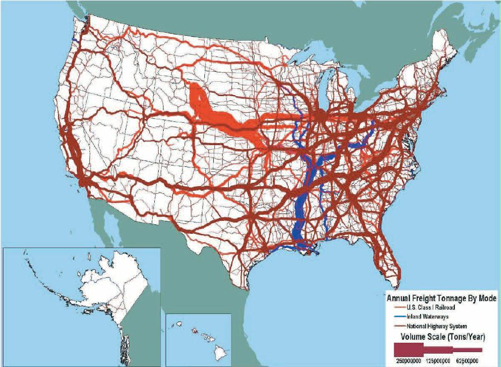
Biggest Waste of Wealth in All of history: America’s Interstate Highway system

A book review by Alice Friedemann of:

Swift, Earl. 2012. The Big Roads: The Untold Story of the Engineers, Visionaries, and Trailblazers Who Created the American Superhighways.

Related articles

Much of what’s below are Swift’s exact or paraphrased words, my comments are italicized. The vast majority of the book is spent on who, what, why, when and where the interstate system was built, but I’ve mainly extracted the bits about energy and material resources, critiques of what the system did to our society, and life before cars. 

Introduction

At 47,000 miles long and four plus lanes wide, the Dwight D. Eisenhower System of Interstate and Defense Highways is the largest public works project in history, dwarfing Egypt’s pyramids, the Panama Canal, and China’s Great Wall.  To build it, forests were felled and mountains were leveled and overlaid with over three hundred million cubic yards of concrete.

Roads are essential and define the physical United States, and so taken for granted they’re almost invisible.

The interstates are just 1% of the nation’s road mileage but carry a trillion of the 4 trillion miles Americans travel each year. Many of the vehicles are heavy trucks, which hammer bridges and pavements, shortening road and bridge lifespans so much that to fix them, we’d need to spend  $225 billion a year for the next 50 years, and if we don’t, replacement will cost three times as much. One in four of the country’s nearly 600,000 bridges is structurally deficient or obsolete. Most were designed to last 50 years. In 2008, they averaged 43 years old (p 319).

Peak Oil Makes Roads and Vehicles Obsolete – Why Fix them?

Swift says that these roads represent “a spectacular investment in a mode of transport that will wither without new fuel sources” (page 6).

We don’t have new fuel sources and never will, so why repair the roads? That would only throw good money after bad. To avoid the hardest possible landing, we might want to keep a few key local and regional roads repaired, and let the thousands of miles of interstate between regions go.  Replace cars with buses, which are flexible, scalable, easily re-routable, and cheap compared to passenger trains since they can use existing roads.

What we have lost  

When horses were the main mode of transportation, American towns were compact, tightly settled, and roughly circular in layout. In the days of the horse and buggy the road served as company. As a cart joggled by, the farmer in the field or the housewife on her porch could hail it; the horse would stop almost of his own accord, and a chat would follow. But once the country road becomes a highway, filled with fast traffic with cars driven mostly by strangers, not neighbors, the whole situation is changed: the road ceases to be a symbol of sociability; it becomes very largely a curse.

As John Steinbeck observed in 1962’s Travels with Charley: In Search of America: “When we get these thruways across the whole country, as we will and must, it will be possible to drive from New York to California without seeing a single thing.”

A pilgrim of centuries past would have had much to report about the country he’d traversed—the details of flora and fauna, the land’s shape and character, the sounds and smells of village and field. He would have noticed the moss on tree bark, the fast-moving stream, the lacework of afternoon light on the forest floor. He might have startled deer and bear, unalerted by his soft approach, or reveled in bird song. A later traveler, riding horseback, might have spoken of the views he’d enjoyed, but they would have been limited views, next to the walker’s. He would have moved at a faster clip, and thus missed the tiny details of his surroundings that only a leisurely pace revealed. Further on, a stagecoach passenger had an even tighter range of experience; he beheld landscape not only from a road’s fixed path, but as a moving picture framed by his window, and his description of a long trip would likely dwell less on the scenery than on the discomforts of the stage, the bumps in the road, the passage itself. Trains erected a pane of glass between traveler and country, and further insulated him by boosting his speed. But with the modern car on the modern freeway, the modern traveler was left with practically nothing to celebrate but the ever-briefer time he had to devote to getting from one place to another. He was sequestered not only from his setting, but from fellow passengers, insulated from sound, smells, and climate. The details of all that surrounded him were blurred by speed, too distant to make out, or too distracting to enjoy. Scenery was held at arm’s length, beyond the well-manicured right of way.

Highways & Roads Ruined our Nation

The messy sprawl of U.S. cities

Destruction of neighborhoods. Clearing a path for the interstates required the taking of more than 750,000 properties.

Boring and predictable chains of fast-food, motels, outlet malls, drive-in banks

Gutting of tens of thousands of small-town shopping districts.  Kunstler describes downtown wastelands in his book The City in Mind: “I remember a spring afternoon I spent as the sole pedestrian in downtown Appleton, Wisconsin, its commercial activity had all been shifted to an asteroid belt of highway strips and architectural garbage five miles outside town.  He describes Atlanta as “a giant hairball of suburbs or ”edge cities,” connected by highways  that has become such a mess nothing can be done to redeem it as a human habitat.”

Shopping Malls. Cookie-cutter malls replaced downtown shopping districts, destroying civic life in exchange for ugly warehouses and vast parking lots. There are no public squares in malls, no public citizenship, just private and lonely consumption of goods from just a few very large corporations that channel wealth to the top one percent of society.

Death

  • In 1929, when a new automobile rolled off an assembly line every six seconds, a life was lost to one of the machines every sixteen minutes.
  • In “The American Way of Death,” Mumford wrote that Americans “are prepared to sacrifice some 59,000 lives every year, and to maim, often irreparably, some three million more.”

The enormous waste of resources for just a few decades of petroleum

  • Cars gobbled vast stores of steel, lead, zinc, rubber, corn, and beeswax; every year the auto industry consumed the wool of seventeen million sheep and the hides of a half-million cattle
  • In 1962 $1 billion was spent on: 16,000,000 barrels of cement, over 500,000 tons of steel, 18,000,000 pounds of explosives, 123,000,000 gallons of petroleum products, enough earth to bury New Jersy knee-deep, and 76,000,000 tons of aggregate– the United States could not mine enough rock to rebuild the interstates today.
  • America spent $130 billion on the interstate highway system. $22 billion of that was fixing Boston’s “Big Dig” array of tunnels and bridges. There are 55,000 bridges, many of them miles long. Maintaining 47,000 miles of highways will cost billions more.
  • Traffic jams cost New Yorkers more than $1 billion a year in fuel, engine wear, lost productivity, missed sales; a quarter of all the gasoline consumed in American cities was burned, it was said, while motorists sat in traffic.

Environmental destruction

  • By 1966 American highways occupied an area the size of West Virginia.
  • Each mile of interstate devoured 30 to 40 acres of farmland; in Iowa alone 710 miles of freeway devoured 26,000 acres of productive cropland–over 40 square miles.
  • Big roads played hell with drainage patterns and water quality. All that concrete encouraged flooding, and salts and oils carried in runoff poisoned nearby ponds and streams and fostered the growth of invasive weeds.
  • Rural interstates presented insurmountable barriers to small mammals, turtles, and amphibians, one study concluding that a 4-lane divided highway was as much a barrier to small creatures as a body of fresh water twice as wide.
  • The slaughter of game by auto approached, and would soon exceed, that by hunting.

We almost used 23 atomic bombs to speed up construction

In 1963, the Atomic Energy Commission and the California State Division of Highways started Project Carryall to determine if atomic bombs could be used to blow up the Bristol mountains near Barstow California, so the I-40 highway and railroad could be built faster and cheaper. The study group of engineers and scientists thought 22 carefully placed atomic bombs would do the trick in a flash with a 36% discount over years of going about it the old way. This would be 60 times as powerful as the Hiroshima and Nagasaki bombs combined. Each bomb packed 20 to 200 kilotons of explosive punch and would vaporize 68 million cubic yards of mountain, creating a chain of connected craters more than two miles long, as much as 340 feet deep, and 330 feet wide at the bottom—plenty big enough for twin railroad tracks and a full-size interstate. A 23rd bomb would blast a reservoir into the desert to collect runoff during storms.

And the engineers promised that there was no need to worry about radioactivity, fallout, air blast, or ground shock because these would be “clean” nuclear explosions. Construction crews could return just 4 days after the explosions.

Lewis Mumford Detested Highways

Mumford was an American historian, sociologist, philosopher of technology, and literary critic. Particularly noted for his study of cities and urban architecture, he had a broad career as a writer.

Cities “worked” not just when they balanced their books, or kept crime off the streets, or picked up the garbage in a timely fashion, but when they fulfilled their more important function of facilitating human interaction—which was, after all, the reason people gathered in cities in the first place. By extension, good architecture incorporated as much sociology as it did engineering or design. A building’s scale and orientation, its relationship to its neighbors, the mood it created in those who beheld it, could fuel a neighborhood’s vitality or hamper it. The width of streets, the presence of trees, the press of high-rises—all were important.

Mumford came to see expressways as wasteful, disruptive, and stupid, absorbing funds badly needed for schools, hospitals, libraries and other facilities.”

He berated highway engineers for behaving “as if motor transportation existed in a social vacuum” and “building more roads, bridges, and tunnels so that more motorcars may travel more quickly to more remote destinations in more chaotic communities, from which more roads will be built so that more motorists may escape from these newly soiled and clotted environments. Our transportation experts are only expert whittlers, and the proof of it is that their end product is not a new urban form but a scattered mass of human shavings. Instead of curing congestion, they widen chaos.”

Mumford passionately believed in the organic aspect of cities, and in their atmosphere, their personality, their feel. New superhighways pumped an ever-heavier flow of cars onto streets and avenues designed for a New York of 4-story buildings. Now “we have in effect piled from three to ten early Manhattans on top of each other. If the average height of these buildings was only twelve stories, the roadway and sidewalks flanking them should, according to the original ratio, be 200 feet wide, the entire width of the standard New York block.”

Mumford attacked the year-old interstate system in 1957, an opening salvo in what would come to be called the Freeway Revolt, making him a darling, to this day, of urban planners, anti-sprawl activists, and critics of the suburban lifestyle. He went straight for the jugular. The interstate program was bound to bring destruction, not salvation, to the nation’s cities. It had been founded “on a very insufficient study” of highways, rather than transportation—on “blunders of one-dimensional thinking”—and would benefit only the “fantastic and insolent chariots” that jammed the streets, “the second mistress that exists in every household right alongside the wife—the motor car.” Want to save the cities? Forget about roads. The solution, Mumford said, lay in restoring a human scale to urban life, in “making it possible for the pedestrian to exist.” A choice was looming, for “either the motor car will drive us all out of the cities, or the cities will have to drive out the motor car.” Americans should “apply our intelligence to the purposes of life,” he said, concluding: “That means eventually we will put the motor car in its place.”

“The wide swathes of land devoted to cloverleafs, and even more complicated multi-level interchanges, to expressways … butcher up precious urban space . They devoured not only open land, but real estate already occupied by people and homes. “Perhaps our age will be known to the future historian as the age of the bulldozer and the exterminator, and in many parts of the country the building of a highway has about the same result upon vegetation and human structures as the passage of a tornado or the blast of an atom bomb. The hell of it was, all that disruption did nothing to ease congestion. Here was a tool that “actually expands the evil it is meant to overcome, and which would continue doing so until that terminal point when all the business and industry that originally gave rise to the congestion move out of the city, to escape strangulation, leaving a waste of expressways and garages behind them.

Mumford concludes with this epitaph: “This is pyramid building with a vengeance: a tomb of concrete roads and ramps covering the dead corpse of a city”.

How did we get here? Don’t blame Detroit Fat Cats: Americans wanted cars

Americans loved everything about their cars, loved driving, loved impulsively going wherever they chose without a thought to routes or timetables. They loved lording over their surroundings while they did it; cocooned, protected from the world, even as they were free to explore it. They could ride in silence or with the radio blaring, need never surrender personal space to a sweaty, foul-smelling stranger or suffer inane chatter. They thrilled to the sensation and sound of movement, the buffet of air through an open window, a big engine’s growl and punch. They embraced the status reflected in chrome trim, the subtext each model offered as to income and station and sex appeal. Americans took to cars not only willingly, but with gusto. They did not have an automotive life foisted on them; they did not buy homes far from work, or forsake mass transit, or pave over their cities because they were manipulated into doing so by Detroit fat cats, or a government-industry conspiracy, or anyone else. No such subterfuge was necessary. The people chose their path. They wanted what they were getting.

Some Cities fought Highways

Too late, San Franciscans realized that they’d permitted a terrible blunder. In place of their waterfront—which, though partially blocked by low buildings, offered one of the most breathtaking urban vistas in the world, overlooking the shimmering bay and Alcatraz Island—they now saw an unadorned gray concrete barricade rising, at its peak, fifty-seven feet from the city’s historic Embarcadero. It cast its surroundings in all-day twilight, severed downtown from the docks that had birthed it, and ran smack across the face of a beloved landmark, the Ferry Building, a gathering spot for generations and a survivor of the 1906 earthquake. To tens of thousands of San Franciscans, the Embarcadero Freeway seemed less a highway than a vivisection. Petitions circulated. Protest groups bloomed. And the public’s outrage was shared by the city fathers: on January 27, 1959, citing “the demolition of homes, the destruction of residential areas, the forced uprooting and relocation of individuals, families and business enterprises,” the Board of Supervisors approved a resolution opposing 7 of the 10 freeways planned for the city, including the yet-unbuilt western two-thirds of I-480. This meant refusing $280 million in Federal Aid money, an unthinkable act in the eyes of most municipal officials. It was a vote heard around the country. Not only did it effectively kill the state’s ambitions for a lavish freeway grid through town, it reverberated with every American confronted by expressways he wasn’t sure he wanted.

Baltimore: Older cities around the country were beset with similar problems, and in each, as in Baltimore, that will was crumbling. A confluence of national trends was shifting the mood of the governed. Historic preservation was becoming a cause beyond the ranks of intelligentsia; Vietnam had created doubt that government knew what it was doing and had the people’s best interests at heart; the civil rights movement had encouraged them to take their grievances to the streets and courts. And perhaps most important, the environmental movement had gained footing among a widening swath of America.

Monotony

Motorists seeking relief from the monotony of the drive found that the system’s sameness wasn’t limited to its right of way, for it wasn’t but a handful of years before the mom-and-pop businesses that had moved out from Main Street were joined by national chains, and the mercantile knots at the exits soon seemed cut from a stencil.

Mom-and-pop businesses on superseded U.S. highways watched their customers vanish as the interstates continued their crawl across the continent. As Florida Trend magazine would cry in 1965, the interstate system “diverts traffic away from former arteries of travel, drains the life’s blood from established firms which are situated on the old highways and leaves them to die.”  Small-town shopping districts weren’t just losing business to the exits, but to bigger towns suddenly made closer by the new highways’ speed and convenience.

What was it about assembly-line food that drew customers by the millions? For starters, it was cheap. But more than that, it answered a growing demand for speed and simplicity. A motorist making good time on the interstate wasn’t inclined to spend time eating a sit-down meal. And the chains’ drive for efficient mass production mirrored a desire in the American public for predictable quality—for preferring the everyday but familiar to a surprise, good or bad.

By 1963, when the interstates were just making tentative inroads into most urban areas, the population of America’s suburbs surpassed that of the cities they ringed. The new houses came fast and cheap, thanks to mass-production techniques that had stamped out hundreds of Liberty ships and thousands of bombers during the war.  James W. Rouse, a Baltimore developer, described the process: “A farm is sold and begins raising houses instead of potatoes, then another farm; forests are cut; valleys are filled; streams are buried in storm sewers; kids overflow the schools; here a new school is built, there a church. Traffic grows; roads are widened; service stations and hamburger stands pockmark the highway. Relentlessly, the bits and pieces of a city are splattered across the landscape.”

In 1966, Americans owned 57% of the world’s passenger cars, drove 922 billion miles, made 92% of their intercity trips by road.

What a shame everyone was smitten with passenger railroads (and still are), when buses make much more sense

Frank Turner was the chief engineer of the interstate system. He was very keen on mass transit, as long as it was provided by bus.  He pointed out that  rail-based transit could not attract enough riders to justify the fortune it would cost to build, because it couldn’t be adapted to changing travel patterns. Cities were spread too far and wide for fixed-rail to take many people from where they were to where they wanted to go. Buses, on the other hand, were extremely flexible. Just 50 or 60 buses could move as many people as 3,000 cars, provide almost door-to-door service, and follow routes that could be adjusted as needed—and they piggybacked on roads already in place, requiring no costly new infrastructure. By boosting the number of buses on the highways, you could actually reduce the need for more highways. Like all his views, his enthusiasm for the bus was supported by research, by statistics. He could cite a 1962 study that showed that buses and subways moved people for about the same cost (3.2 cents per person per mile) but that buses were far, far cheaper to put into service. He could point to 1968 research that showed a single express lane devoted to buses could move the same number of commuters as four lanes of freeway.

Turner could not fathom why environmentalists, the press, and anti-highway activists didn’t embrace the bus, or why they were so smitten with rail-based transit. The “infinite combinations of routes and schedules required by today’s urban dwellers dictates that any transportation system must provide flexibility of route, destination and schedules. That’s why fixed-route systems which are basically spoke lines attached to a downtown hub have such a hard time financing themselves in the fare box.

His detested the Washington Metro, that initially covered 98 miles and cost about $3 billion ($4,000 per household), an amount equal to everything spent on the capital region’s roads since the beginning of  settlement there. “What a huge capital expenditure to provide for the movement of about 5% of the transportation load within Washington’s metropolitan area. Just the annual interest on the debt would buy about 5,000 new buses every year for the whole life of Metro”.

Roads started because of demands from bicyclists

In 1874, overland travel was done by train. Look at any state and you’d see tangles of thick black lines converging on the major cities. Most of the old maps don’t depict a single road. They were there, but hardly in the form we think of them. The routes out of most any town in America were “wholly unclassifiable, almost impassable, scarcely jackassable,” as folks said then—especially when spring and fall rains transformed the simple dirt tracks into a heavy muck, more glue than earth. People braved roads to the train and back, or to roll their harvest from their farms to the nearest grain elevator. For any trip beyond that, they went by rail.

Some of the first bicycles had enormous front and tiny rear wheels, with saddles perched as high as 5 feet off the ground. On steep downhills, the best a rider could do was brace his feet on the handlebars, so that if he crashed, the bike stopped cold, with calamitous results, if that big front wheel encountered an obstacle— he’d at least go flying right-side up.

At local bicycle ships and meetings of the national organization the League of American Wheelmen, there were always conversation’s about cycling’s most urgent need: roads on which to ride.  Bicycling was a jarring experience in the 1890s, even when city streets were paved with cobblestone, brick, or uneven granite block, and snarled with carts, buggies, and horsemen. Outside the business districts, roads dwindled to little more than wagon ruts. A sprinkling of rain could turn them to bogs; their mud lay deep and loose, could suck the boots off a farmer’s feet, prompting travelers to quit the established path for the open fields. Some muddy roads swallowed horses to their flanks; the unfortunate buggy that ventured down such a lane soon flailed past its axles in the ooze. Even on hard-packed roads, mud formed dark rooster tails behind surreys, spattered long skirts, caked shoes. American business was conducted in mud-soiled suits, as were law, medicine, and church services. And mixed with the mud was a liberal helping of manure, for city and country alike were dependent on the horse.

Cyclists thus found their hobby not as pleasant as it could be, and the League of American Wheelmen committed to doing something about it. Their magazine, Good Roads,  became an influential mouthpiece for road improvement. Its articles were widely reprinted, which attracted members who didn’t even own bikes; eventually there were 102,000 subscribers, and the Good Roads Movement was too big for politicians to ignore. The demand for roads was pedal-powered, and a national cause even before the first practical American car rolled out of a Chicopee, Massachusetts, shop in 1893.

A few months ahead of the Duryea Motor Wagon’s debut, Congress authorized the secretary of agriculture to “make inquiry regarding public roads” and to investigate how they might be improved. So it was that in October 1893, agriculture secretary J. Sterling Morton created the Office of Road Inquiry and appointed to head it one Gen. Roy Stone, a Civil War veteran, civil engineer, and vociferous good roads booster from New York. His appointment was the sort of circular affair—a lobbyist pushing for government action that he winds up leading. Stone considered it “settled” that Americans “have the worst roads in the civilized world,” and that their condition was “a crushing tax on the whole people, a tax the more intolerable in that it yields no revenue.” Spending nothing on bad roads cost more than spending money to make them better, he argued, in squandered productivity, spoiled crops, high food prices.

America’s first overland routes started out as game trails

America’s principal overland routes were descended from prehistory— they’d started as game trails, had been commandeered by Native American hunting parties, and later were widened into wagon roads by white settlers. Over decades of use, they’d been cleared of stumps—at least the big ones—but much of their engineering remained the work of buffalo and elk. Improving on that was no easy matter.

Most roads were bare-dirt scars flanked by deep and weedy ditches. The newer ones had high crowns, their edges sloping downhill from their centers to drain water, but it wasn’t long before they were mashed into concavity and diabolically rutted. Some highways were dragged, meaning that after a rain a neighboring landowner would hitch a horse to a rig of split logs and pull it over the ruts to flatten them out. Rebuilding a road consisted of shoveling dirt from its sides into the middle, then tamping it down. Grading with a horse-drawn blade was a cause for local celebration.

How the first roads were built (also see “Why is modern concrete falling apart?”)

A concentration of heavy freight wagons, or “horse trucks,” had forced cities to pave their business districts, but the stone used for the purpose was far too expensive for rural roads built and maintained by county and local governments, which had little income and could tax their citizens only so much. Rains turned rural roads into quagmires. Even the best country road of the early twentieth century was primitive. The most common “improvement” was simply to grade a dirt road’s surface, in an attempt to smooth its bumps and fill its ruts. A step up was sand-clay construction, for which a mix of the two soils would be imported and spread on an earthen bed; the result in theory, was a surface that drained well and with traffic achieved a smooth hardness, but it also broke down quickly under heavy loads.

A little better was the gravel road, on which river rock or broken stone was spread on a graded bed; it held up better than dirt, especially to horse traffic, but had to be dressed regularly to keep the gravel from scattering, and it was stripped bare by the skinny tires and higher speeds of cars and trucks.

The most popular solution to that dilemma was macadam. It pre-dated the automobile by nearly 80 years after it was noticed gravel highways didn’t become smooth and durable until a lot of traffic had compressed their stone into a unified, interlocking mass. In 1816 a smooth dirt bed was covered with a ten-inch layer of stone broken especially for the purpose by workers armed with small hammers, then passed over the rock with a heavy, horse-drawn roller. The sharp-edged stones knitted into a tight bond. American road builders refined his system by spreading a thick layer of large broken stone onto graded earth, rolling it, covering it with a second layer of much smaller stone, and rolling it again. The surface with rock dust, hosed down with water, and rolled it a third time. “Water-bound macadam,” this was called, and it performed well under normal loads and low speeds. To keep dust down, workers topped it with a thin layer of asphalt, a black, sticky, molasses-like petroleum goop or coal-derived tar, which also kept the rock in place. The roads of today are asphaltic concrete, a blend of asphalt or tar and an aggregate, or filler, most commonly broken rock or gravel.

Why people were eager to switch from horses to cars and trucks

Horses required stabling, feed, and health care, which nationally amounted to $2 billion a year, or as much as it cost to maintain all of America’s railroads. Feeding the typical horse consumed five acres of tillable land a year; devoted to food for people, the nation’s feed-producing cropland could support millions [more people]. Horses are slow and can’t keep going fast for long and need frequent rest, food, water. Horses had to work seven times as hard on a dirt road as on a hard, smooth rock surface, and asphalt and brick offered even easier going.

Eisenhower does not deserve the credit for the interstate system

These highways didn’t come from Eisenhower. Long before June 1956, most of its physical details were old news. Its routing had already been nailed down for18 years and design-specifics for 12. FDR had a greater hand in its creation than Eisenhower, and the system’s origins go back much further than even FDR. The true parents were anonymous career technocrats. If the system bore the name of the man most responsible for its existence, it would be called the Thomas H. MacDonald System of Interstate and Defense Highways, who conceived of the network and proposed its construction before World War II.


Posted in Concrete, Infrastructure Books, Roads, Transportation, Transportation Infrastructure, Trucks | Tagged , , , | Comments Off on Biggest Waste of Wealth in All of history: America’s Interstate Highway system

Wind notes from government studies

[These are here to help me do research and find citations]

Notes from 96 page: EERE. August 2014. 2013 Wind technologies market report. Energy Efficiency & Renewable Energy.

No commercial offshore turbines have been commissioned in the United States, but offshore project and policy developments continued in 2013. At the end of 2013, global offshore wind capacity stood at roughly 6.8 GW.

The United States also had the capability of producing approximately 7 GW of blades and 8 GW of towers annually. Despite the significant growth in the domestic supply chain over the last decade, prospects for further expansion have dimmed. More domestic wind manufacturing facilities closed in 2013 than opened. Additionally, the entire wind energy sector employed 50,500 full-time workers in the United States at the end of 2013, a deep reduction from the 80,700 jobs reported for 2012

Independent power producers own 95% of the new wind capacity installed in 2013. [My note: this is why it’s so hard to get true figures to come up with a realistic EROI, because this data is private and when data is shared with scientists, may be from the best performing windfarms, since this could lead to more investment money coming in].

Operations and maintenance costs varied by project age and commercial operations date Operations and maintenance costs are a significant component of the overall cost of wind energy and can vary substantially among projects. Anecdotal evidence and recent analysis (Lantz 2013) suggest that unscheduled maintenance and premature component failure in particular continue to be key challenges for the wind power industry. Given the scarcity, limited content, and varying quality of the data, the results that follow may not fully depict the industry’s challenges with O&M issues and expenditures.

Lack of transmission can be a barrier to new wind power development, and insufficient transmission capacity in areas where wind projects are already built can lead to curtailment, as illustrated earlier. New transmission is particularly important for wind energy because wind power projects are constrained to areas with adequate wind speeds, which are often located at a distance from load centers. There is also a mismatch between the relatively short timeframe often needed to develop a wind power project compared to the longer timeframe typically required to build new transmission. Uncertainty over transmission siting and cost allocation, particularly for multi-state transmission lines, further complicates transmission development.

Moreover, on a cumulative basis considering all wind installed in the United States by the end of 2013, independent power producers (IPPs) own 83% of wind power capacity, while utilities own 15%, with the final 2% owned by entities that are neither IPPs nor utilities (e.g., towns, schools, commercial customers, farmers). On a cumulative basis, utilities own (15%) or buy (54%) power from 69% of all wind power capacity in the United States, with merchant/quasi-merchant projects accounting for 23% and competitive power marketers 8%.

Technology Trends • Turbine nameplate capacity, hub height, and rotor diameter have all increased significantly over the long term. The average nameplate capacity of newly installed wind turbines in the United States in 2013 was 1.87 MW, up 162% since 1998–1999. The average hub height in 2013 was 80 meters, up 45% since 1998-1999, while the average rotor diameter was 97 meters, up 103% since 1998–1999.

Growth in rotor diameter has outpaced growth in nameplate capacity and hub height in recent years. Rotor scaling has been especially significant in recent years, and more so than increases in nameplate capacity and hub heights, both of which have seen a modest reversal of the long-term trend in the most recent years. In 2012, almost 50% of the turbines installed in the United States featured rotors of 100 meters in diameter or larger. Though 2013 was a slow year for wind additions, this figure jumped to 75% in that year.

Turbines originally designed for lower wind speed sites have rapidly gained market share. With growth in average swept rotor area outpacing growth in average nameplate capacity, there has been a decline in the average “specific power” i (in W/m2) among the U.S. turbine fleet over time, from 400 W/m2 among projects installed in 1998–1999 to 255 W/m2 among projects installed in 2013. In general, turbines with low specific power were originally designed for lower wind speed sites. Another indication of the increasing prevalence of lower wind speed turbines is that, in 2012, more than 50% of installations used IEC Class 3 and Class 2/3 turbines; in 2013, based on the small sample of projects installed that year, the percentage increased to 90%.

Trends in sample-wide capacity factors have been impacted by curtailment and inter-year wind resource variability. Wind project capacity factors have generally been higher on average in more recent years (e.g., 32.1% from 2006–2013 versus 30.3% from 2000–2005), but time-varying influences—such as inter-year variations in the strength of the wind resource or changes in the amount of wind power curtailment—have tended to mask the positive influence of turbine scaling on capacity factors in recent years.

Competing influences of lower specific power and lower quality wind project sites have left average capacity factors among newly built projects stagnant in recent years, averaging 31 to 34 percent nationwide. Even when controlling for time-varying influences by focusing only on capacity factors in 2013 (parsed by project vintage), it is difficult to discern any improvement in average capacity factors among projects built after 2005

The average quality of the wind resource in which new projects are located has declined; this decrease was particularly sharp—at 15%—from 2009 through 2012.

Regional variations in capacity factors reflect the strength of the wind resource and adoption of new turbine technology. Based on a sub-sample of wind projects built in 2012, average capacity factors in 2013 were the highest in the Interior (38%) and the lowest in the West (26%).

Not surprisingly, these regional rankings are roughly consistent with the relative quality of the wind resource in each region.

Recently announced turbine transactions have often been priced in the $900–$1,300/kW range. [My comment: So a typical 2 MW turbine (2,000 kW) would cost $1.8 to $2.6 million dollars, and so replacing a 500 MW fossil-powered plant would cost $450 million to $650 million dollars, and last 20 years rather than the 35 year lifespan of natural gas and coal plants]

Operations and maintenance costs varied by project age and commercial operations date. Despite limited data availability, it appears that projects installed over the past decade have, on average, incurred lower operations and maintenance (O&M) costs than older projects in their first several years of operation, and that O&M costs increase as projects age.

Policy and Market Drivers

Availability of Federal incentives for wind projects built in the near term has helped restart the domestic market, but policy uncertainty persists. In January 2013, the PTC was extended, as was the ability to take the 30% investment tax credit (ITC) in lieu of the PTC. Wind projects that had begun construction before the end of 2013 are eligible to receive the PTC or ITC. These provisions have helped restart the domestic wind market and are expected to spur capacity additions in 2014 and 2015. With the PTC now expired and its renewal uncertain, however, wind deployment beyond 2015 is also uncertain.

2013 Wind Technologies Market Report

State policies help direct the location and amount of wind power development, but current policies cannot support continued growth at recent levels. As of June 2014, RPS policies existed in 29 states and Washington D.C. From 1999 through 2013, 69% of the wind power capacity built in the United States was located in states with RPS policies; in 2013, this proportion was 93%. However, given renewable energy growth over the last decade, existing RPS programs are projected to require average annual renewable energy additions of just 3–4 GW/year through 2025 (only a portion of which will be from wind), which is well below the average growth rate in wind capacity in recent years, demonstrating the limitations of relying exclusively on RPS programs to drive future deployment.

[My comment: it appears that wind turbines depend on government subsidies, implying a low EROI]

Solid progress on overcoming transmission barriers continued. Over 3,500 miles of transmission lines came on-line in 2013, a significant increase from recent years. Four transmission projects of particular importance to wind, including the Competitive Renewable Energy Zones project in Texas, were completed in 2013. A decrease in transmission investment is anticipated in 2014 and 2015.

System operators are implementing methods to accommodate increased penetration of wind energy. Recent studies show that wind energy integration costs are almost always below $12/MWh—and often below $5/MWh—for wind power capacity penetrations of up to or even exceeding 40% of the peak load of the system in which the wind power is delivered.

Because federal tax incentives are available for projects that initiated construction by the end of 2013, significant new builds are anticipated in 2014 and 2015. Near-term wind additions will also be driven by the recent improvements in the cost and performance of wind power technologies, leading to the lowest power sales prices yet seen in the U.S. wind sector. Projections for 2016 and beyond are much less certain. Despite the lower price of wind energy and the potential for further technological improvements and cost reductions, federal policy uncertainty—in concert with continued low natural gas prices, modest electricity demand growth, and the aforementioned slack in existing state policies—may put a damper on growth.

The report concentrates on larger-scale wind turbines, defined here as individual turbines that exceed 100 kW in size.1 The U.S. wind power sector is multifaceted, however, and also includes smaller, customer-sited wind turbines used to power residences, farms, and businesses. Data on these smaller turbines are not the focus of this report, although a brief discussion on Smaller Wind Turbines is provided on page 4.

The U.S. wind power market slowed dramatically in 2013, with only 1,087 MW of new capacity added, bringing the cumulative total to 61,110 MW (Figure 1).3 This growth required $1.8 billion of investment in wind power project installations in 2013, for a cumulative investment total of $125 billion since the beginning of the 1980s (all cost and price data are reported in real 2013$).4

The table below summarizes sales of smaller (100-kW and smaller) wind turbines into the U.S. market from 2003 through 2013. As shown, 5.6 MW of small wind turbines were sold in the United States in 2013, with 88% of that capacity coming from U.S. suppliers (Orrell and Rhoads-Weaver 2014). These installation figures represent a very substantial decline in sales relative to recent years. The average installed cost of U.S. small wind turbines in 2013 was reportedly $6,940/kW

Annual Sales of Smaller Wind Turbines (= 100 kW) Year into the United States Capacity Additions Number of Turbines 2003 3.2 MW 3,200 2004 4.9 MW 4,700 2005 3.3 MW 4,300 2006 8.6 MW 8,300 2007 9.7 MW 9,100 2008 17.4 MW 10,400 2009 20.4 MW 9,800 2010 25.6 MW 7,800 2011 19.0 MW 7,300 2012 18.4 MW 3,700 2013 5.6 MW 2,700 Source: Orrell and Rhoads-Weaver (2014) Sales in this sector historically have been driven—at least in part—by a variety of state incentive programs. In addition, wind turbines of 100 kW or smaller are eligible for an uncapped 30% federal investment tax credit (ITC, in place through 2016). The Section 1603 Treasury Grant Program and programs administered by the U.S. Department of Agriculture have also played a role in the sector. According to AWEA (2014a), competitive PV and natural gas prices, suspended state incentives, and a weak economy have all contributed to recent declines in sales.

With the drop-off in annual wind power capacity additions in 2013, wind power’s share of total U.S. electric generation capacity additions in that year shrank to 7% (Figure 2).5 Overall, wind power ranked fourth in 2013 as a source of new generation capacity, behind natural gas (48% of total U.S. capacity additions), solar (26%), and coal (10%). This diminished contribution stands in stark contrast to 2012 when wind power represented the largest source of new capacity in the United States, and it marks a notable divergence from the six years preceding 2013 during which it constituted between 25% and 43% of capacity additions in each year.

Led by the decline in the U.S. market, global wind additions contracted to approximately 36,000 MW in 2013, 20% below the record of roughly 45,000 MW added in 2012. Cumulative global capacity stood at approximately 321,000 MW at the end of the year (Navigant 2014; Table 1).6 The United States ended 2013 with 19% of total global wind power capacity, a distant second to China by this metric (Table 1).7 Annual growth in cumulative capacity in 2013 was 2% for the United States and 13% globally. After leading the world in annual wind power capacity additions from 2005 through 2008, and then losing the mantle to China from 2009 through 2011, the United States narrowly regained the global lead in 2012. In 2013, however, the United States dropped precipitously to 6th place in annual wind additions (Table 1).

The U.S. wind power market represented just 3% of global installed capacity in 2013. The top five countries in 2013 for annual capacity additions were China, Germany, India, the UK, and Canada. Table 1. International Annual Capacity (2013, MW) China 16,088 Germany 3,237 India 1,987 United Kingdom 1,833 Canada 1,599 United States 1,087 Brazil 948 Poland 894 Sweden 724 Romania 695 Rest of World 7,045 TOTAL 36,137 Cumulative Capacity (end of 2013, MW) China 91,460 United States 61,110 Germany 34,468 Spain 22,637 India 20,589 United Kingdom 10,946 Italy 8,448 France 8,128 Canada 7,813 Denmark 4,747 Rest of World 51,031 TOTAL 321,377

A number of countries have achieved relatively high levels of wind energy penetration in their electricity grids. Figure 4 presents data on end-of-2013 (and earlier years’) installed wind power capacity, translated into projected annual electricity supply based on assumed country-specific capacity factors and then divided by projected 2014 (and earlier years’) electricity consumption. Using this approximation for the contribution of wind power to electricity consumption, and focusing only on those countries with the greatest cumulative installed wind power capacity, end-of-2013 installed wind power is estimated to supply the equivalent of 34% of Denmark’s electricity demand and approximately 20% of Spain, Portugal and Ireland’s demand. In the United States, the cumulative wind power capacity installed at the end of 2013 is estimated, in an average year, to equate to almost 4.5% of the nation’s electricity demand. On a global basis, wind energy’s contribution is estimated to be 3.4%.

On a cumulative basis, Texas remained the clear leader among states, with 12,354 MW installed at the end of 2013—more than twice as much as the next-highest state (California, with 5,829 MW). In fact, Texas has more installed wind capacity than all but five countries (including the United States) worldwide. States (distantly) following Texas in cumulative installed capacity include California, Iowa, Illinois, Oregon, and Oklahoma—all with more than 3,000 MW. Thirty-four states, plus Puerto Rico, had more than 100 MW of wind capacity installed as of the end of 2013, with 23 of these topping 500 MW, 16 topping 1,000 MW, and 10 topping 2,000 MW. Although all commercial wind projects in the United States to date have been installed on land,

The right half of Table 2 lists the top 20 states based on actual wind electricity generation in 2013 divided by total in-state electricity generation in 2013.9 Iowa and South Dakota lead the list, each with more than 25% wind penetration. A total of nine states have achieved wind penetration levels of above 12% of in-state generation.

Wind energy penetration can either be expressed as a percentage of in-state load or in-state generation. In-state generation is used here, primarily because wind energy (like other energy resources) is often sold across state lines, which tends to distort penetration levels expressed as a percentage of in-state load.

Annual (2013) California 269 Kansas 254 Michigan 175 Texas 141 New York 84 Nebraska 75 Iowa 45 Colorado 32 Ohio 3 Massachusetts 3 Alaska 3 North Dakota 2 Indiana 1 Puerto Rico 1 Rest of U.S. 0 TOTAL 1,087 Table 2. U.S. wind power rankings: the top 20 states Percentage ofInstalled Capacity (MW)In-State Generation

Cumulative (end of 2013) Actual (2013)* Texas California Iowa Illinois Oregon Oklahoma Minnesota Kansas Washington Colorado New York North Dakota Indiana Wyoming Pennsylvania Michigan Idaho South Dakota New Mexico Montana Rest of U.S. TOTAL 12,354 Iowa 27.4% 5,829 South Dakota 26.0% 5,177 Kansas 19.4% 3,568 Idaho 16.2% 3,153 Minnesota 15.7% 3,134 North Dakota 15.6% 2,987 Oklahoma 14.8% 2,967 Colorado 13.8% 2,808 Oregon 12.4% 2,332 Wyoming 8.4% 1,722 Texas 8.3% 1,681 Maine 7.4% 1,544 California 6.6% 1,410 Washington 6.2% 1,340 New Mexico 6.1% 1,163 Montana 6.0%

One testament to the continued interest in land-based wind energy is the amount of wind power capacity currently working its way through the major transmission interconnection queues across the country. Figure 7 provides this information for wind power and other resources aggregated across 37 different interconnection queues administered by independent system operators (ISOs), regional transmission organizations (RTOs), and utilities.11 These data should be interpreted with caution: although placing a project in the interconnection queue is a necessary step in project development, being in the queue does not guarantee that a project actually will get built. Efforts have been made by FERC, ISOs, RTOs, and utilities to reduce the number of speculative projects that have—in recent years—clogged these queues. One consequence of those efforts, as well as perhaps the uncertain size of the future U.S. wind market, is that the total amount of wind power capacity in the nation’s interconnection queues has declined dramatically since 2009.

Much of the wind capacity in the interconnection queues is planned for Texas, the Midwest, Southwest Power Pool (SPP), PJM Interconnection, the Northwest, the Mountain region, and California; wind power projects in the interconnection queues in these regions at the end of 2013 accounted for 95% of the aggregate 114 GW of wind power in the selected queues (Figure 8). Smaller amounts of wind power capacity were represented in the interconnection queues of ISONew England (ISO-NE, 2.5%), the New York ISO (NYISO, 1.9%), and the Southeast (0.7%).

Manufacturing facilities that produce multiple components are included in multiple bars. “Other” includes facilities that produce items such as: Enclosures, composites, power converters, slip-rings, inverters, glass prepeg, electrical components, tower internals, climbing devices, couplings, castings, steel, rotor hubs, plates, walkways, doors, bearing cages, fasteners, bolts, magnetics, safety rings, struts, clamps, fiberglass, transmission housings, embed rings, electrical cable systems, yaw/pitch control systems, bases, generator plates, slew bearings, lubrication, resin, flanges, anemometers, template rings. Source: National Renewable Energy Laboratory Figure 11. Number of operating wind turbine and component manufacturing facilities in the United States Five of the ten wind turbine OEMs with the largest share of the U.S. market through 2013 (GE, Vestas, Siemens, Gamesa, Acciona) had one or more manufacturing facilities in the United States at the end of 2013. In contrast, nine years earlier (2004), there was only one active utility-scale wind energy OEM assembling nacelles in the United States (GE).15 In 2013, however, several of the OEMs’ manufacturing facilities were largely if not entirely dormant given the lack of turbine orders, and at least one of these facilities was subsequently closed in 2014. Another major OEM, Nordex, ceased U.S. manufacturing in 2013, while several others stopped U.S. manufacturing in past years (e.g., Clipper and Suzlon). In aggregate, domestic turbine nacelle assembly capability—defined here as the maximum nacelle assembly capability of U.S. plants if all were operating at maximum utilization—grew from less than 1.5 GW in 2006 to exceed 12 GW in 2012, before dropping to roughly 10 GW in 2013 (Figure 12;

Manufacturing facilities that produce multiple components are included in multiple bars. “Other” includes facilities that produce items such as: Enclosures, composites, power converters, slip-rings, inverters, glass prepeg, electrical components, tower internals, climbing devices, couplings, castings, steel, rotor hubs, plates, walkways, doors, bearing cages, fasteners, bolts, magnetics, safety rings, struts, clamps, fiberglass, transmission housings, embed rings, electrical cable systems, yaw/pitch control systems, bases, generator plates, slew bearings, lubrication, resin, flanges, anemometers, template rings.

Figure 14 presents calendar-year data on the dollar value of estimated imports to the United States of wind-related equipment that can be tracked through trade codes. Specifically, the figure shows imports of wind-powered generating sets (i.e., nacelles not surprisingly, taller towers have seen higher market share in the Great Lakes (56%) and Northeast (43%) than in the Interior (7%) and West (3%). This is largely due to the fact that such towers are most commonly used in lower wind speed sites, and presumably those with higher wind shear, to access the better wind speeds that are typically higher up.

Figure 31. Average cumulative sample-wide capacity factor by calendar year Table 5.

Inter-Year Wind Resource Variability. The strength of the wind resource varies from year to year, in part in response to significant persistent weather patterns such as El Niño/La

Competing influences of lower specific power and lower quality wind project sites have left average capacity factors among newly built projects stagnant in recent years, averaging 31 to 34 percent nationwide

Counterbalancing the decline in specific power, however, has been a tendency to build new wind projects in lower-quality wind resource areas; this is especially the case among projects installed from 2009 through 2012.

the average estimated quality of the wind resource at 80 meters among projects built in 2012 (i.e., the most recent project vintage in our capacity factor sample included in figure 32) is roughly 15% lower than it is among projects built back in 1998–1999 and that the decline has been particularly sharp since 2008.45 Although there was a bit of a rebound in 2013 (which will impact our sample in future years), this trend of building wind power projects in progressively lower-quality wind resource areas is a key reason why overall average capacity factors have not increased for projects installed in recent years. The trend may also come as a surprise, given that the United States still has an abundance of undeveloped high-quality wind resource areas.

Several factors could be driving this trend:

Technology Change. The increased availability of low-wind-speed turbines that feature higher hub heights and a lower specific power may have enabled the economic build-out of lower-wind-speed sites. Transmission and Other Siting Constraints. Developers may have reacted to increasing transmission constraints (or other siting constraints, or even just regionally differentiated wholesale electricity prices) by focusing on those projects in their pipeline that may not be located in the best wind resource areas but that do have access to transmission (or higher priced markets, or readily available sites without long permitting times).

Policy Influence. Projects built in the 4-year period from 2009 through 2012 were able to access a 30% cash grant (or ITC) in lieu of the PTC. Because the dollar amount of the grant (or ITC) was not dependent on how much electricity a project generates, it is possible that developers seized this limited opportunity to build out the less-energetic sites in their development pipelines. Additionally, state RPS requirements sometimes require or motivate in-state or in-region wind development in lower wind resource regimes.

Berkeley Lab has gathered price data for 112 U.S. wind turbine transactions totaling 29,250 MW announced from 1997 through the beginning of 2014, including ten transactions (2,082 MW) announced in 2013/14. Sources of turbine price data vary, including SEC and other regulatory filings, as well as press releases and news reports. Most of the transactions included in the Berkeley Lab dataset include turbines, towers, delivery to site, and limited warranty and service agreements.48 Nonetheless, wind turbine transactions differ in the services included (e.g., whether towers and installation are provided, the length of the service agreement, etc.), turbine characteristics (and therefore performance), and the timing of future turbine delivery, driving some of the observed intra-year variability in transaction prices.


Unfortunately, collecting data on U.S. wind turbine transaction prices is a challenge: only a fraction of the announced turbine transactions have publicly revealed pricing data. In part as a result, Figure 38—which depicts these U.S. wind turbine transaction prices—also presents data from: (1) Vestas on that company’s global average turbine pricing from 2005 through 2013, as reported in Vestas’ financial reports; and (2) a range of recent global average wind turbine prices for both older turbine models (smaller rotors) and newer models (larger rotors), as reported by Bloomberg NEF (2014b).

After hitting a low of roughly $750/kW from 2000 to 2002, average wind turbine prices increased by approximately $800/kW (more than 100%) through 2008, rising to an average of more than $1,500/kW. The increase in turbine prices over this period was caused by several factors, including a decline in the value of the U.S. dollar relative to the Euro; increased materials, energy, and labor input prices; a general increase in turbine manufacturer profitability due in part to strong demand growth and turbine and component supply shortages; increased costs for turbine warranty provisions; and an up-scaling of turbine size, including hub height and rotor diameter (Bolinger and Wiser 2011).

our limited sample of recently announced U.S. turbine transactions shows pricing in the $900–$1,300/kW range. Bloomberg NEF (2014b) reports global average pricing for the most-recent contracts of approximately $1,000/kW for older turbine models and $1,300/kW for newer turbine models that feature larger rotors.

In aggregate, the dataset (through 2013) includes 708 completed wind power projects in the continental United States totaling 50,210 MW and equaling roughly 82% of all wind power capacity installed in the United States at the end of 2013.

Operations and maintenance costs varied by project age and commercial operations date Operations and maintenance costs are a significant component of the overall cost of wind energy and can vary substantially among projects. Anecdotal evidence and recent analysis (Lantz 2013) suggest that unscheduled maintenance and premature component failure in particular continue to be key challenges for the wind power industry.

Figure 44 shows an upward trend in project-level O&M costs as projects age, although the sample size after year 5 is limited. In addition, the figure shows that projects installed more recently (from 2005–2008 and/or 2009-2012) have had, in general, lower O&M costs than those installed in earlier years (from 1998–2004), at least for the first 8 years of operation. Parsing the “recent project” cohort into two sub-periods, however, reveals that this trend towards lower costs has not necessarily continued with the most recent projects in the sample, those installed from 2009-2012 (though cost differences between the 2005-2008 and 2009-12 sample are small and sample size is limited).


Many of the projects installed more recently may still be within their turbine manufacturer warranty period, and/or may have capitalized O&M service contracts within their turbine supply agreement.

As indicated previously, the data presented in Figures 43 and 44 include only a subset of total operating expenses. In comparison, the financial statements of public companies with sizable U.S. wind project assets indicate markedly higher total operating costs. Specifically, two companies—Infigen and EDP Renováveis (EDPR), which together represented approximately 4,730 MW of installed capacity at the end of 2013 (nearly all of which has been installed since 2000)—report total operating expenses of $24.2/MWh and $23.6/MWh, respectively, for their U.S. wind project portfolios in 2013 (EDPR 2014, 2013, 2012; Infigen 2014, 2013, 2012, 2011).59 These total operating expenses are more than twice the $10/MWh average O&M cost reported above for the 85 projects in the Berkeley Lab data sample installed since 2000.

This disparity in operating costs between these two project owners and the Berkeley Lab data sample reflects, in large part, differences in the scope of expenses reported.

Important Note: Notwithstanding the comparisons made in this section, neither the wind nor wholesale electricity prices (nor fuel cost projections) reflect the full social costs of power generation and delivery. Specifically, the wind PPA prices are reduced by virtue of federal and, in some cases, state tax and financial incentives. Furthermore, these prices do not fully reflect integration, resource adequacy, or transmission costs.

Various policy drivers at both the federal and state levels have been important to the expansion of the wind power market in the United States, as have been federal investments wind energy research and development (R&D). In addition to R&D expenditure, at the federal level, the most important policy incentives in recent years have been the PTC (or, if elected, the ITC), accelerated tax depreciation, and an American Recovery and Reinvestment Act of 2009 (Recovery Act) provision that enabled wind power projects to elect, for a limited time, a 30% cash grant in lieu of the PTC.

First established in 1992, the PTC provides a 10-year, inflation-adjusted credit that stood at 2.3¢/kWh in 2013.

The historical importance of the PTC to the U.S. wind power industry is illustrated by the pronounced lulls in wind power capacity additions in the 4 years (2000, 2002, 2004, 2013) in which the PTC lapsed as well as the increased development activity often seen during the year in which the PTC is otherwise scheduled to expire (see Figure 1); the spike in wind additions in 2012 is a clear example of this latter effect.

Accelerated tax depreciation enables wind project owners to depreciate the vast majority of their investments over a 5- to 6-year period for tax purposes. An even more attractive 50% 1st-year “bonus depreciation” schedule was in place during 2008–2010. Legislation in midDecember 2010 further increased 1st-year bonus depreciation to 100% for those projects placed in service between September 8, 2010 and the end of 2011, after which the 1st-year bonus reverted to 50% for projects placed in service during 2012. The American Taxpayer Relief Act then extended this 50% bonus depreciation for qualifying property placed in service in 2013 (and 2014 for certain long-lived property).

From 1999 through 2013, 69% of the wind power capacity built in the United States was located in states with RPS policies; in 2013, this proportion was 93%.66 As of June 2014, mandatory RPS programs existed in 29 states and Washington D.C. (Figure 50).67

In aggregate, existing state RPS policies require that by 2025 (at which point most state RPS requirements will have reached their maximum percentage targets) at least 9% of total U.S. generation supply will be met with RPS-eligible forms of renewable electricity, equivalent to roughly 106 GW of renewable generation capacity.68 Incremental growth in RPS requirements through 2025 represents 40% of projected growth in total U.S. electricity generation over that timeframe, although some portion of the growth in RPS requirements may be met with existing capacity (e.g., in regions that are currently over-supplied relative to their RPS targets).

Given the size of RPS targets and the amount of new renewable energy capacity that has been built since enactment of those policies, Berkeley Lab projects that existing state RPS programs require average annual renewable energy additions of roughly 3–4 GW/year through 2025, not all of which will be wind.69 This is below the average of 7 GW of wind power capacity added in each year over the 2007–2013 period, and even further below the 9 GW per year of total renewable generation capacity added during that time frame, demonstrating the limitations of relying exclusively on state RPS demand to drive future wind power development.

WA: 15% by 2020 MN: 26.5% by 2025ME: 40% by 2017MT: 15% by 2015 Xcel: 31.5% by 2020 NH: 24.8% by 2025 ND: 10% by 2015 MI: 10% by 2015 VT: 20% by 2017MA: 11.1% by 2009 +1%/yrOR: 25% by 2025 (large utilities) 5-10% by 2025 (smaller utilities) SD: 10% by 2015 WI: 10% by 2015 NY: 30% by 2015RI: 16% by 2019 PA: 8.5% by 2020 NV: 25% by 2025 IA: 105 MW by 1999 CT: 23% by 2020 NJ: 22.5% by 2020DE: 25% by 2025 OH: 12.5% by 2024 UT: 20% by 2025 KS: 20% of peak IL: 25% by 2025 demand by 2020 CO: 30% by 2020 (IOUs) MO: 15% by 2021CA: 33% by 2020 20% by 2020 (co-ops) 10% by 2020 (munis)OK: 15% by 2015 AZ: 15% by 2025 NM: 20% by 2020 (IOUs) 10% by 2020 (co-ops) AK: 50% by 2025 DC: 20% by 2020 MD: 20% by 2022 VA: 15% by 2025 NC: 12.5% by 2021 (IOUs) 10% by 2018 (co-ops and munis) TX: 5,880 MW by 2015 HI: 40% by 2030 Mandatory RPS Non-Binding Goal Source: Berkeley Lab

State renewable energy funds provide support for wind power projects (both financial and technical) in some jurisdictions, as do a variety of state tax incentives.

Transmission development has gained traction in recent years. FERC reports that over 3,500 miles of transmission lines came on-line in 2013, a significant increase from recent years (Figure 51). Another 15,000 miles of transmission lines are in various stages of development with a proposed on-line date of 2016 or earlier, with about one-third of those lines having a high probability completion (FERC 2014). According to the Edison Electric Institute (EEI), total transmission investment by investor-owned utilities reached $17.5 billion in 2013. EEI forecasts a decrease in investment in 2014 and 2015, primarily attributable to recent economic conditions and the continuance of low electric demand growth. Nonetheless, EEI identified over 170 transmission projects in development representing more than $60 billion in possible investment, 76% of which would—at least in part—support the integration of renewable energy (EEI 2014).

One of the most significant transmission undertakings devoted to wind power, the Competitive Renewable Energy Zones (CREZ) project in Texas, was largely finished by the end of 2013. The CREZ includes almost 3,600 circuit miles of transmission lines and was designed to accommodate up to 18,500 MW of total wind power capacity, 11,500 MW of which is additional to what existed when the lines were planned in 2008.70 The $6.8 billion cost of CREZ was $2 billion higher than first estimated, in part because over 600 circuit miles of additional transmission lines were needed to accommodate requested changes in routing from landowners. Because of CREZ, ERCOT reports that wind-related congestion between West Texas and other zones has largely disappeared. Moreover, ERCOT predicts that over 7,000 MW of new wind capacity will be installed in Texas by the end of 2015, with another 1,300 MW projected to come online in 2016. ERCOT recently issued a report stating that projected wind development in the Texas Panhandle is exceeding expectations, and additional transmission, reactive power and synchronous condensers will need to be added (ERCOT 2014). Partly in response, the Texas PUC has opened a staff investigation on whether any such costs should be assigned to renewable energy generators rather than to all customers, as is currently the case (Texas PUC 2014).


Elsewhere, NV Energy and Great Basin Transmission South, an affiliate of LS Power, completed the 236 mile, 500-kV, One Nevada transmission project that connects NV Energy and Sierra Pacific Power. LS Power is also developing two other transmission projects: the 500-kV Southern Nevada Intertie Project and the 500-kV Southwest Intertie Project North, both of which in combination with the ON Line could transmit over 2,000 MW. Two other transmission projects of importance to wind that were completed in 2013 include: (1) the Montana-Alberta Tie Line, a 230-kV merchant transmission line capable of transmitting 300 MW that connects Alberta to Northwestern Energy in Montana; and (2) the Pawnee-Smoky Hill double-circuit, 345-kV transmission line between the cities of Brush and Aurora in Colorado, which can transmit 300 to 500 MW of generation.

Due to the variable nature of wind, considerable attention is paid to the potential impacts of wind energy on power systems. Concerns about, and solutions to, these issues have affected, and continue to impact, the pace of wind power deployment in the United States. Experience in operating power systems with wind energy is also increasing worldwide, leading to an emerging set of best practices (Exeter and GE 2012, WGA 2012).

Figure 52 provides a selective listing of estimated wind integration costs associated with increased wind energy from integration studies completed from 2003 through 2013 at various levels of wind power capacity penetration. With one exception, wind integration costs estimated by the studies reviewed are below $12/MWh—and often below $5/MWh—for wind power capacity penetrations up to and even exceeding 40% of the peak load of the system in which the wind power is delivered. Variations in estimated costs across studies are due, in part, to differences in methodologies, definitions of integration costs, power system and market characteristics, wind energy penetration levels, fuel price assumptions, and the degree to which thermal power plant cycling costs are included.

Note also that the rigor with which the various studies have been conducted varies, as does the degree of peer review.

Finally, there has been some recent literature questioning the methods used to estimate wind integration costs and the ability to disentangle those costs explicitly, with up to 30% of PJM’s energy coming from wind and solar, given adequate transmission expansion and additional regulating reserves.

Posted in Wind | Comments Off on Wind notes from government studies

$46 Trillion Infrastructure in USA, $6 Trillion is Transportation

James Howard Kunstler has written that Suburbia will be the largest waste of money and physical assets in human history.

The end of the age of oil means that just about everything will be useless too.  Below is just the transportation component of private and government assets.

$6.1 Trillion dollars of Transportation equipment and structures.

Total private and public fixed assets were $46.4 trillion in 2011 (current U.S. dollars). Transportation equipment and structures (private and public) accounted for nearly 12% percent of the total.

The components of transportation fixed assets and their values are

  • private transportation equipment ($1.04 trillion)
  • private transportation structures ($680 billion)
  • government transportation structures ($3.77 trillion)

Fixed assets include both passenger and freight transportation. See the Bureau of Economic Analysis at www.bea.gov/national/FA2004/index.asp, tables 2.1, 3.1s, and 7.1b.

2011
Private Sector
Transportation Equipment1 1,037
Transportation Structures2 680
Public Sector
Highways 3,132
Transportation Structures2 635
Federal 15
State and Local 621


1 Includes trucks, truck trailers, buses, automobiles, aircraft, ships, boats, and railroad equipment.

2 Includes physical structures for all modes of transportation. Source: U.S. Department of Commerce, Bureau of Economic Analysis, National Economic Accounts, Fixed Assests Tables, tables 2.1, 3.1s, and 7.1b

Posted in Transportation Infrastructure | Tagged , | 1 Comment

Gail Tverberg: How this collapse differs from past collapses

Converging Energy Crises – And How our Current Situation Differs from the Past

At the Age of Limits Conference, I gave a talk called Converging Crises (PDF), talking about the crises facing us as we reach energy limits. In this post, I discuss some highlights from a fairly long talk.

A related topic is how our current situation is different from past collapses.

The Nature of our Current Crisis

Figure 1

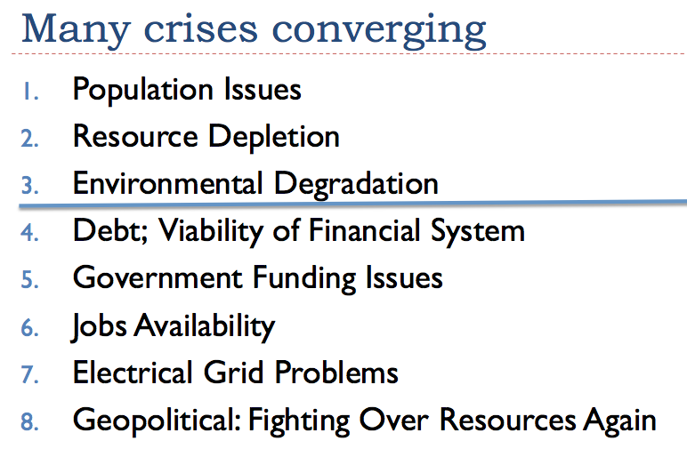
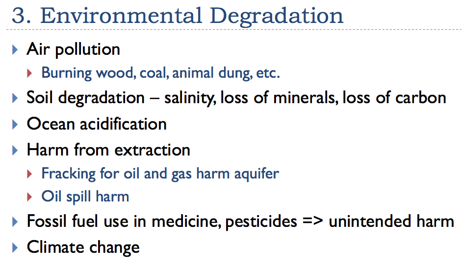
The first three crises are the basic ones: population growth, resource depletion, and environmental degradation. The other crises are not as basic, but still may act to bring the system down.

Figure 2

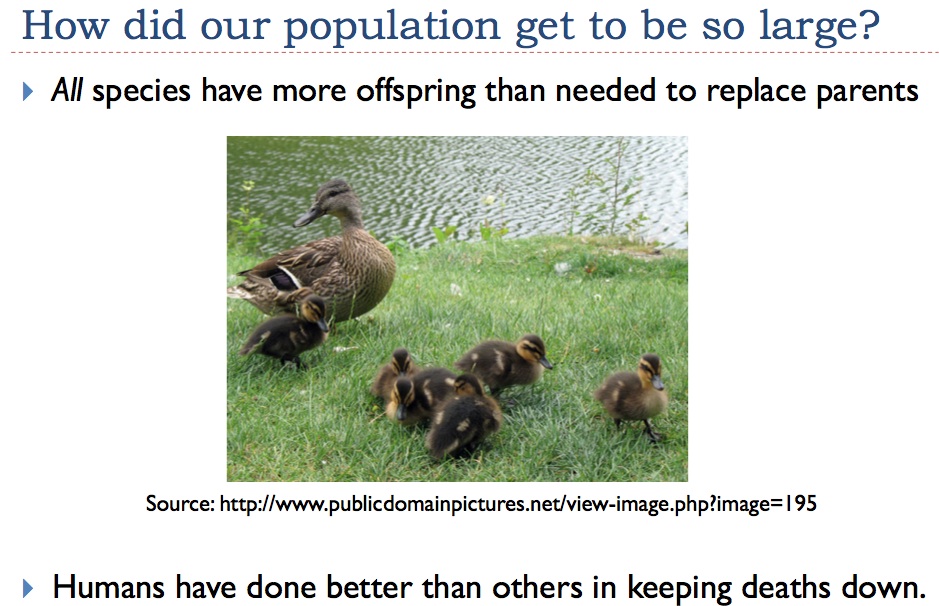
Humans have found a series of ways to keep deaths down, each adding more control of external energy.

  • Control of fire, starting over 1 million years ago. This allowed humans to cook their food, making it possible for more energy to go to develop the brain, and less to developing teeth and digestive apparatus. Humans could also extend their range into colder areas.
  • Agriculture, starting about 10,000 years ago. We grew desirable plants and animals and excluded other species, thus increasing the amount of food produced.
  • Coal, starting around 1800 C. E. With coal, we could make metals in quantity since we didn’t need to cut down trees for smelting. We could also make concrete and glass in quantity. With these, we could build hydroelectric power plants, and build electric transmission lines.
  • Oil, ramping up after World War II. Oil allowed the use of cars for personal transport, plus trucks to deliver goods precisely where they were needed. It also improved agricultural productivity through irrigation, refrigeration, herbicides, pesticides. The ability to use airplanes enabled globalization.

As humans’ control of energy improved, human population grew and the population of other species fell. According to Niles Eldredge, the Sixth Mass Extinction began 100,000 years ago, when there were fewer than 100,000 people on the planet, back in the days of hunter-gatherers. The extent of die-off of other species has grown as we added agriculture, and later added coal and oil use.

Humans are not doing anything “wrong.” Humans are reacting to the same instinct that all species have, namely to make use of available energy to allow more of the species to live to maturity. Population growth stops when a species reaches a limit of some sort–lack of food because the species eats too much of its would-be food supply; too much pollution; epidemics (related to crowding and poor nutrition); or limits associated with gathering external energy.

Individuals can change their personal actions, but built-in instincts tend to guide the direction of civilizations as a whole. Thus the population of civilizations tend to rise until bottlenecks are reached.

Resource Depletion is Particularly a Problem for Oil

We are seeing depletion in many areas right now, including fresh water aquifers, soil erosion, the number and size of fish in the ocean, the number of pollinators, and deforestation. The mineral concentration of ores we are mining keeps getting lower as well. For the purpose of the talk, I will concentrate on oil, however.

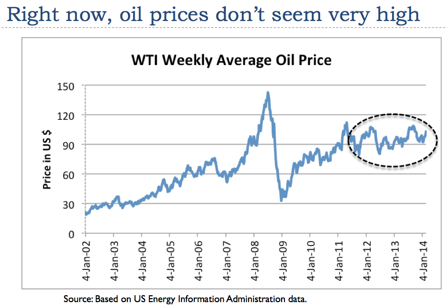
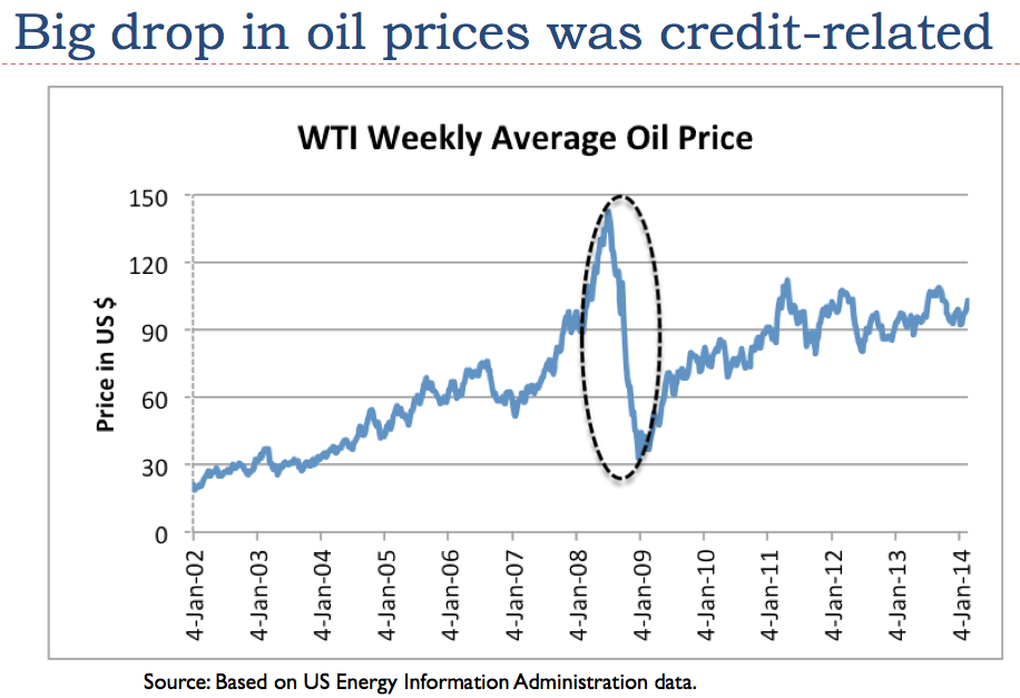
Right now, oil is suffering from depletion but prices don’t seem very high.

Figure 3.

The cost of extracting oil keeps rising, whether or not the prices consumers pay rise, because the cheapest to extract oil was pulled out first. The problem now is that oil prices are too low for producers, at the same time that they are very high for the consumer. The low prices for producers mean that oil companies must take extraordinary measures, such as adding more debt, or selling land they planned to develop, to have enough money to pay dividends. Companies extracting oil from shale formations are in particularly tough shape because they tend to be small and have poor credit ratings.

The low-price oil situation looks likely to reach a crisis stage in the near term. What has been holding the situation together is today’s low interest rates. With these low interest rates, investors who are desperate for higher yields will invest in “iffy” companies, like shale oil companies. In addition, oil producing companies can borrow at low rates, helping to keep costs down.

It is hard to see a fix for the problem oil producing companies are now having. If oil prices rise to help them, consumers will find that the higher oil prices “squeeze” their discretionary income. As a result, we will be pushed back into recession. So no oil price works.

How Decline in Oil Supply Can Be Expected to “Work”

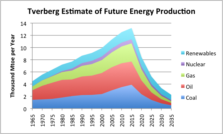
Many people are of the view that if oil production declines, it will decline slowly, more or less over the same time-period it rose, in a symmetric “Hubbert” Curve. My expectation is that the downslope will be much steeper than the upslope. I also expect that all fuels will fall in use, more or less simultaneously. This pattern occurs because of the networked way the world economy is constructed and because of the role of debt, which I will describe later.

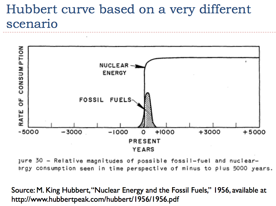
The Hubbert Curve was constructed in the special case where another fuel took over before fossil fuels started to decline (Figure 4), a situation which does not exist today.

Figure 4

In my view, a more realistic view of the expected downslope is shown in Figure 5, below.

Figure 5. Estimate of future energy production by author. Historical data based on BP adjusted to IEA groupings.

It is my expectation that the supply of all fuels will decrease in use, more or less together, because of credit related financial problems that will affect the economy as a whole.

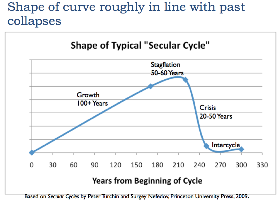
Peter Turchin and Surgey Nefedov analyzed how eight agricultural civilizations collapsed  in the book Secular Cycles. First, there is a long period of growth and population expansion, as the group makes increasing use of a new resource available (such as land cleared for agriculture). This is followed by a “stagflation” period of 50 to 60 years after population reaches the carrying capacity of the new resource. Stagflation is followed by a crisis period of 20 to 50 years, when debt defaults became common, governments collapse, and population decreases. I show this pattern in Figure 6, below.

Figure 6

My forecast energy downslope in Figure 5 is  intended to follow roughly the shape of the curve of prior collapses, depicted in Figure 6. The sharpness of the points in Figure 6 occur because I plotted only 5-year points–annual points would have produced a smoother curve.

Environmental Degradation Takes Many Forms

Figure 7

The environmental degradation issue that gets the most “press” is climate change. If any one limit is modeled, whether it is soil problems, or the mass extinction of many species that seems to be currently taking place, or ocean acidification, it is likely to show that that particular problem is likely to take civilization down. To get a balanced view of what is ahead, a person would need to model all limits at once.

Climate change modelers are of course mainly interested in their limit. They have started to incorporate some information of the effect of other limits into the “low end” of their range (that is, the 2.6 degree scenario), but the “high estimate”–which gets much of the press–assumes no limits of any other sort. It includes far more carbon from fossil fuels than seems reasonable, in my view.

The Financial System is Terribly Important, and Debt Problems Can Bring it Down

Today’s economy is a network of interconnected businesses and consumers, regulated by governments. The financial system is extremely important to this network. In a way, the financial system is like the operating system of a computer. It telegraphs what products are needed, where, and what resources are available to meet these needs from one part of the economy to another. It allows businesses to profitably meet these needs.

Debt plays a surprisingly important role in our current economy. Increasing the amount of debt available increases the amount of goods a person can buy. For example, if a consumer has a job paying $40,000 a year, and gets a loan for $20,000 to buy a new car, the effect is similar to having $60,000 in income for that year. Similarly, if a business can borrow money for a new factory, it can add to jobs to the economy.

When the growth in debt turns to contraction (this happens if consumers default in large numbers, or if they buy fewer homes and cars), it has a huge impact on the economy. The shrinking debt tends to push the economy into contraction. Because there is less demand for commodities like oil, coal and natural gas, the prices of these commodities tend to fall. In fact, a credit contraction seems to be precisely what happened in July 2008, when oil prices took a steep drop. Prices of other fuels also dropped at the same time.

Figure 8

In fact, since 2008, the US economy is still struggling with inadequate growth in debt. The underlying reason is that consumers’ wages are lagging, so they cannot afford more debt. The government tries to make up for the lack of growth in consumer debt by borrowing more money itself and by keeping interest rates artificially low, through Quantitative Easing.

A basic underlying issue is the fact that our salaries don’t rise as oil prices rise. Similarly, our salaries don’t rise with rising interest rates. Both oil prices and interest rates very much affect what need to pay, however. Oil prices affect food and transportation costs, and interest rates affect mortgage and auto loan payments. If interest rates rise again, or if oil prices rise, many consumers will be forced to cut back on discretionary spending. As a result, the economy is likely to shift back into recession. Prices of commodities such as oil, gas, coal, and uranium are likely to fall again.  Ultimately production of these commodities can be expected to fall, because without debt, they become unaffordable for most consumers.

Government Funding Issues

One issue noted by Turchin and Nefedov is that in prior collapses, government funding is generally a problem. This occurs because the government is funded by surpluses of an economy. If an economy is reaching diminishing returns, citizens find it harder and harder to get good-paying jobs at the same time that the government needs more funding to handle the problems it is confronting, such as the need for a larger army. As a result, it becomes very hard to collect enough taxes. If tax rates are raised too high, citizens find themselves unable to afford an adequate diet. With poor nutrition, citizens become more vulnerable to epidemics–one of the major causes of die-offs in collapses.

We are seeing the issue of inadequate government funding now. US publicly held debt has been soaring since mid 2008 (Figure 9).

Figure 9

Inadequate High-Paying Jobs Go with Too Little Energy

Figure 10

An early sign of lack of adequate energy is a lack of good-paying jobs for young people. Also, the jobs that are available tend to be low-paying service jobs that don’t require much energy.

Of course, if we have to go back to growing food without today’s energy inputs, there will be a huge number of manual labor jobs available. But these are not the jobs most people are thinking about.

Electrical Grid Problems

Figure 11

There is a popular myth that electricity will save us. This view is based on the view that our problem is simply a liquid fuels problem. Our problem is really very much deeper–a systems problem that threatens to take down the financial system and the consumption of all types of fuels simultaneously. Thus, the same problems that bring down oil consumption threaten to bring down electricity consumption.

But even apart from the systems problem, it is clear that oil problems lead to electric grid  problems. The electric grid needs constant repairs. New parts must be transported using oil, and the supply lines of companies manufacturing these parts must continue to operate, again using oil. Trucks or helicopters using oil products are needed to put grid replacement parts in place. Workers need transportation for their work on the grid, as well.

The claim that wind and solar PV will save us is silly, if we have an unsolvable grid problem. The place for solar PV is off-grid. Wind also works off-grid, in uses such as pumping water. Of course, wind turbines used for this purpose are tiny compared to today’s electricity generating turbines.

Geopolitical Problems

Figure 12

As we become more resource constrained, we can expect more fighting among countries. Perhaps new alliances will  be formed, in an attempt to squeeze our current energy hogs–US, Europe, and Japan. It is possible that the US dollar will lose its status as reserve currency, leading to a lower standard of living for US citizens.

Solutions to Converging Crises

Figure 13

You may think I am kidding with respect to the last item, “We need help from a Higher Power,” but I am not. Our universe seems to have been created by a Big Bang. But big bangs don’t just happen. We live in a very orderly universe. According to Newton’s Laws of Motion, for every action, there is an equal and opposite reaction. We also know that useful energy is balanced by friction. This, in fact, is a necessary balance, or the system would spin out of control. We also would not be able to drive down the road in a car without friction.

If a big bang happened, it seems likely to me that there was a major force behind the big bang. We can call this force Nature or a Higher Power. I am doubtful that the force behind the big bang would fix the world situation so that humans can continue along their current destructive path on earth. But the force might fix the situation in some other way–perhaps make the transition for humans easier to bear, or produce a new kind of big bang supporting an afterlife for humans as envisioned by various religions.

How This Time is Different

Greer, in his talk, mentioned several points about prior collapses:

  • Typically 95% of the population died off.
  • The time between civilizations tended to be about 500 years.
  • The 5% who survived were able to go about doing things, pretty much as had been done in the past.
  • The downslopes often had jogs and bumps in them, and could be slow.

The question arises as to how helpful this information is with respect to what is ahead. As I see the situation, civilizations that failed in the past were not fossil fuel dependent or electricity dependent. While there was specialization of labor, there was much less specialization than there is today. While there was some trade, the majority of food and clothing was locally produced. The biggest problems were

  • Growing population
  • Arable farmland that did not expand to meet growing population
  • Soil problems (loss of fertility, erosion, salinity)
  • Deforestation
  • Competition from neighboring civilizations
  • Government collapse
  • Debt problems

I view the 500 year gap between civilizations as including what I show as the “inter cycle” period between civilizations in Figure 6, above. This is the gap that took place before new growth could occur.

The big problem in the past with civilizations that collapsed was that humans were using renewable resources faster than they could renew. Population continued to expand as well. The combination of rising population and depleting soil and forest resources led to diminishing returns, lower wages for many workers, and difficulty funding governments. A 500 year gap between civilizations took the population pressure off an area. Forests were able to regrow, and soil was able to renew (at least partly through regeneration of soil by erosion of base rock).

Today, we sill have the problems we had in the past, but we have some new ones as well:

  • We are depleting aquifers much more rapidly than they regenerate. In many cases, the water table is far below what can be reached with simple tools. It will take thousands of years for these aquifers to regenerate.
  • We are depleting minerals of all kinds, so that we now need “high tech” methods to extract the low ore concentrations. These minerals will be out of reach, without the use of electricity and fossil fuels. In fact, the vast majority of fossil fuel energy supplies will also be out of reach, without today’s high tech methods. Eventually this may change, with new fossil fuel formation and with earthquakes, but the timeframe is likely to be millions of years.
  • Most people today do not know how to live without fossil fuels and electricity. If fossil fusel and electricity disappeared, most of us would not know how to produce our own food, water, and other basic necessities.
  • Most of us could not just “pick up and do as we did before,” with respect to our current jobs, if the government and 95% of the population disappeared. Our jobs are often supported by global supply chains that would disappear, as well as direct use of fossil fuels and electricity.
  • The world is sufficiently networked that most of it is likely to be drawn into a world-wide collapse. In the past, areas that did not collapse continued to function. These areas could act as a back-up, if functions were lost.

In the past, the 500 year gap was enough to allow regeneration of forests and soil, once population pressures were reduced. If that were our only problem now, we could expect the same pattern again. Such a regeneration would allow a reasonably large group of people (say 500 million people) to get back to a non-fossil fuel based civilization in 500 years, with new governments, roads and other services.

In such a new civilization, we would likely have difficulty using much metals, because ores are now quite depleted. Even reprocessing of existing metals is likely to require more heat energy than is easily available from renewables sources.

We are now so dependent on fossil fuels and electricity that any collapse that does take place seems likely to be faster than prior collapses. If the electric grid goes down in an area, and cannot be repaired, most business functions will be lost–practically immediately. If oil supply is interrupted, it also will bring a halt to most business in an area, because workers can’t get to work and raw materials cannot be transported.

We are bing told, “Renewables will save us,” but this is basically a lie. Wind and solar PV are just as much a part of our current fossil fuel system as any other source of electricity. They will only last as long as the weakest link–inverters that need replacing, batteries that need replacing, or the electric grid that needs fixing. We are being told that these are our salvation, because politicians need to have something to point to as a solution–not because they really will work.

Posted in Crash Coming Soon, Gail Tverberg | Tagged , , | Comments Off on Gail Tverberg: How this collapse differs from past collapses

Exponential growth examples

Monbiot, George. 27 May 2014. It’s simple. If we can’t change our economic system, our number’s up It’s the great taboo of our age – and the inability to discuss the pursuit of perpetual growth will prove humanity’s undoing. The Guardian.

Imagine that in 3030 BC the total possessions of the people of Egypt filled one cubic meter, which grew 4.5% a year. How big would that stash have been 3,000 years later?   2.5 billion billion solar systems   (That’s 2.5 quadrillion, or 2,500,000,000,000,000,000).

Ignore if you must climate change, biodiversity collapse, the depletion of water, soil, minerals, oil; even if all these issues miraculously vanished, the mathematics of compound growth make continuity impossible.

Economic growth is an artifact of the use of fossil fuels. Before large amounts of coal were extracted, every upswing in industrial production would be met with a downswing in agricultural production, as the charcoal (from wood) or horse power required by industry reduced the land available for growing food. Every prior industrial revolution collapsed, as growth could not be sustained. But coal broke this cycle and enabled – for a few hundred years – the phenomenon we now call sustained growth.

It was neither capitalism nor communism that made possible the progress and pathologies (total war, the unprecedented concentration of global wealth, planetary destruction) of the modern age. It was coal, followed by oil and gas. The mother narrative, is carbon-fueled expansion. Our ideologies are mere subplots. Now, with the accessible reserves exhausted, we must ransack the hidden corners of the planet to sustain our impossible proposition. The scouring of the planet has only just begun–everywhere that contains something concentrated, unusual, precious, will be sought out and exploited, its resources extracted and dispersed, the world’s diverse and differentiated marvels reduced to the same grey stubble.

Some people try to solve the impossible equation with the claim that as processes become more efficient and gadgets are miniaturized, we use, in aggregate, fewer materials. There is no sign that this is happening. Iron ore production has risen 180% in 10 years. The trade body Forest Industries tells us that “global paper consumption is at a record high level and it will continue to grow”. If, in the digital age, we won’t reduce even our consumption of paper, what hope is there for other commodities?

Look at the lives of the super-rich, who set the pace for global consumption. Are their yachts getting smaller? Their houses? Their artworks? Their purchase of rare woods, rare fish, rare stone? Those with the means buy ever bigger houses to store the growing stash of stuff they will not live long enough to use. Ever more of the surface of the planet is used to extract, manufacture and store things we don’t need. Perhaps it’s unsurprising that fantasies about colonizing space – which tell us we can export our problems instead of solving them – have resurfaced.

The inescapable failure of a society built upon growth and its destruction of the Earth’s living systems are the overwhelming facts. As a result, they are mentioned almost nowhere. They are the 21st century’s great taboo, the subjects guaranteed to alienate your friends and neighbors. We live as if trapped inside a Sunday supplement: obsessed with fame, fashion and the three dreary staples of middle-class conversation: recipes, renovations and resorts. Anything but the topic that demands our attention.

Statements of the bleeding obvious, the outcomes of basic arithmetic, are treated as exotic and unpardonable distractions, while the impossible proposition by which we live is regarded as so sane and normal and unremarkable that it isn’t worthy of mention. That’s how you measure the depth of this problem: by our inability even to discuss it.


Posted in Exponential Growth, Limits To Growth | 2 Comments

Expressways & Interstates are only designed to last for 20 years

Figure 2-5. Tonnage on U.S. highways, railroads, and inland waterways (U.S. Department of Transportation FHWA FM&O 2007).

Figure 2-5. Tonnage on U.S. highways, railroads, and inland waterways (U.S. Department of Transportation FHWA FM&O 2007).

Preface. I make the case that civilization would end in a week if trucks stopped running in my first book, and though I had in mind that they would be running low on diesel fuel on the downside of world peak oil production, if roads fall apart as well, and can’t be maintained because of lack of energy, that’ll stop trucks as well.

Roads are Essential

There are 4,016,741 miles of roads in the United States.  The most critical roads are the almost 47,000 miles long with 55,000 bridges and 4 or more lanes wide Interstate Highways, the largest single investment the American people have made in public works.

Over eleven million trucks worth $1 Trillion dollars deliver goods over these roads. Trucks moved nearly 70% of all domestic freight — 9.4 billion tons of stuff. If you put all of these trucks in a line, it would stretch from the earth to the moon over 11 times.

According to the most recent information from the Commodity Flow Survey (CFS), on average, 42 tons of freight worth $39,000 was delivered to every person in the United States in 2007 transported an average of 11,000 ton-miles to every person in the country.

Since railroads are on average 4.5 to 6.5 times more energy efficient than trucks in ton miles of freight moved per gallon (Tolliver) it’s a shame, no, a crime, that there are only 140,000 miles of railroad tracks (down from 254,000 miles in 1916), just 3.5% of the 4 million road miles. Freight trains used 2% of our petroleum. Trucks burned 46% — 20% medium and heavy trucks (classes 3-8) burned 20% and 26% light trucks another (CTA).

Do you like to eat?  Here’s how grain is typically moved from point A to point B (bold represents diesel burning vehicles).  After harvesting the grain it’s trucked to on-farm storage, then trucked to a country elevator, then the grain moves by truck or train from the country elevator to the sub-terminal elevator,  then a train or barge delivers the grain to the export elevator, and the grain is loaded on a ship and taken to the destination country.

Roads are in Bad Shape

But they’re falling apart and need $930 billion of work. Driving on this poor pavement costs motorists an additional $67 billion in vehicle repairs and operating costs every year (ASCE). When you consider all the ways highways are assaulted, it’s not hard to see why.

Heavy Trucks

According to the AASHO Road Test, heavy trucks can do more than 10,000 times the damage of a car. The amount of damage varies by how fast the truck is going, how uneven the road is, and many other factors (Hjort).

Soil, weather, & exponential growth

The freeze-thaw cycle cracks, swells, and buckles pavement.  Roads fissure from heat, depressions grooved by wheels, abrasion of studded tires, water filling cracks and freezing, water and salt corroding steel rebar. Roads unravel from lost surface stones, potholes, and poor maintenance.

The amount of traffic today is often more than double what the road was originally designed for. No one thought freight would move from trains to roads given how much more fuel efficient trains are, and engineers can’t anticipate the new suburbs and shopping malls that flood highways with more vehicles.

Local materials affect longevity

Concrete is the most heavily used substance in the world after water (Sedgwick), which is why gravel, crushed stone, and sand are the leading items transported by weight – one in seven tons of freight. But they don’t go far, the average distance moved is 60 miles, because the shipping is so expensive and their value so low.

This means that often less than ideal local material is used to make concrete.

Roads are two to four foot thick cakes, with six layers (Subgrade, capping, sub-base, binder course, and the frosting is the surface course). Each layer is baked with local materials, and never with the same recipe — there are an infinite number of recipes. Adding to the limitless permutations is what kind of steel is used, since steel varies in what alloys were used, and how strong, resistant to corrosion, and easily welded it is. Asphaltic concrete only adds to the mystery, since it has an unknown chemistry brought in by the source of the crude oil it was derived from (Skinner).

Roads can last longer

They’re designed to last for 40 years in some European countries with thicker, more durable roadbeds using concrete rather than asphalt. Concrete lasts longer, but it costs more and takes longer to repair. Asphalt is cheap and fast, but falls apart quickly.

Longer Lasting Roads are Expensive

Long-lasting roads are much thicker and cost more, which need more money up front, and taxpayers tend to object to that. Look what it took to make Chicago’s 30-year Dan Ryan Expressway at a cost of $1 billion per 10 miles (Adams):

  • Old road: 27 inches thick. 12 inch aggregate., 10 inch concrete. 5 inch asphalt.
  • New road: 44 inches thick. 24 inch aggregate. 14 inch concrete. 6 inch asphalt.

The United States has numerous agencies who’ve come up with ways to build longer lasting roads, but this often requires new equipment, which small construction and paving companies can’t afford, and the majority of highway construction is done by small firms.

Highway agencies have fixed budgets, so even though it would cost far less in the long run to make a 50-year-road, they often don’t have the money at the outset to pay for a better road. Highway agencies also try to build and maintain the maximum number of miles possible and don’t want to blow their wad on relatively few miles of highway, even if that would be the best use of public funds.

There are no incentives to build long-lasting low maintenance roads. Politicians get no immediate political return from building long-lasting roads, low-bidders usually get the work so quality suffers, and financing is done by cost per mile, not durability per mile over time. On top of all that, the number of pavement design engineers is shrinking from downsizing, retirement, and young engineers not being attracted to this field.

Peak Oil – the End of Roads?

Peak oil is an awful lot like losing your job with no hope of new one ever again. It’s not a good time to buy a new car, you’ll need every penny of your savings to pay for food, housing, insurance, and utilities.

We’ve been at peak oil since 2005 and any day now could slide down the other side of Hubbert’s peak.  It’s an awful time to replace 11 million trucks worth $1 trillion dollars and millions of miles of underground pipelines that deliver diesel fuel across the nation with something else that doesn’t even exist yet.

And if you did that, then what?  The roads are falling apart.  Swift writes “Bringing the system into full repair, and keeping it there, will cost us $225 billion a year for the next 50 years to rehabilitate surface transportation. What’s at stake, ultimately, is a foundation of America’s safety, economy, and mobility since we do 96% of our traveling by car and truck. And not making the fixes will wind up costing more as needed repairs balloon into reconstruction. “If we can get this work done now,” said John Horsley, AASHTO’s executive director, “it will cost one-third of what it’ll cost if we put things off.”

Swift concludes that this highway system “represents a spectacular investment in a mode of transport that will wither without new fuel sources….Before long, we’ll be compelled to develop a wholesale replacement for gasoline. We’d better hope we do, anyway. Because without alternative fuels, we may see the interstates morph from the world’s biggest highway system into its biggest white elephant”.

A few more statistics

  • In 2008, 4.5 million people were employed in transportation and warehousing industries in the United States, a little over 3% of total U.S. employment.
  • Trucking was the largest employer within the for-hire transportation section with almost 1.4 million employed.
  • The railroad industry employed 231,000.  There are 94,942 miles of Class I freight railroad tracks, 46,474 miles of regional and shortline railroad tracks
  • water transportation employed 67,000.There are 26,000 miles of navigable inland waterways
  • Another key component of logistics services and supply chains, warehousing and storage, employed 672,000

Alice Friedemann  www.energyskeptic.com Women in ecology  author of 2021 Life After Fossil Fuels: A Reality Check on Alternative Energy best price here; 2015 When Trucks Stop Running: Energy and the Future of Transportation”, Barriers to Making Algal Biofuels, & “Crunch! Whole Grain Artisan Chips and Crackers”.  Podcasts: Crazy Town, Collapse Chronicles, Derrick Jensen, Practical Prepping, KunstlerCast 253, KunstlerCast278, Peak Prosperity

References

ASCE (American Society of Civil Engineers). 2013. Report Card: Roads.

Adams, C. Dec 31, 2010. Why don’t roads last longer? StraightDope.com

CTA. Center for Transportation Analysis. 2013. Transportation Energy Data book Edition 32. Chapter 2. Energy. Oak Ridge National Laboratory.

Hjort, Mattias, et al. Road wear from Heavy Vehicles – an overview. Report nr. 08/2008 NVF committee Vehicles and Transports.

Preserving and Protecting Freight Infrastructure and Routes. 2012. National Academy of Sciences.

Sedgwick, J. 1991. Strong but sensitive. Atlantic Monthly, April 1991, pp. 70–82.

Skinner Jr., R.E. 2008. Highway Design and Construction: The Innovation Challenge. National Academy of Engineering.

Tolliver, D, et al. May 2013. Analysis of Railroad Energy Efficiency in the United States.

Upper Great Plains Transportation Institute, North Dakota State University

U.S. Department of Transportation RITA/BTS 2010, Table 3-19b

Additional reading

Gibbons, J. 1999. Pavements and Surface Materials. University of Connecticut Nonpoint education for municipal officials technical paper #8.

Keller, G et al. July 2003. Low-volume roads engineering. Chapter 12. Roadway Materials and Material Sources for Low Volume Roads. USDA Forest service.

Swift, Earl. The Big Roads: The Untold Story of the Engineers, Visionaries, and Trailblazers Who Created the American Superhighways.

Posted in Infrastructure & Fast Crash, Roads, Trucks | Tagged , , , , , | 2 Comments

My Favorite James Howard Kunstler podcasts

You can subscribe to these on iTunes, or go to http://kunstler.com/writings/podcast/

I haven’t listened to all of his podcasts yet, these are the ones I’ve best liked so far (I’ve left a lot of good ones out):

KunstlerCast 253 – Yakking with Alice Friedemann of EnergySkeptic.com

Alice Friedemann insists she is not an academic, but publishes on a wide variety of contemporary scientific issues bearing on the fate of industrial civilization. She subscribes to a scenario that she calls the “fast crash.” She worked for 25 years as a systems architect and engineer in the corporate world, or “Dilbert-Land” as she calls it, before dropping out to write full time. Her science and economic essays can be found at her website: Energyskeptic.com. Alice is also a cookbook writer and blogger at the website Wholegrainalice.com She lives in Berkeley, California.
Direct Download:  http://traffic.libsyn.com/kunstlercast/KunstlerCast_253.mp3

KunstlerCast 241 — Snake Oil: Richard Heinberg on the Great Shale Snooker

JHK yaks with Richard Heinberg about his new book, Snake Oil: How Fracking’s False Promises of Plenty Imperils Our Future. Richard is also the author of the great peak oil primer, The Party’s Over, and many other books about the converging dilemma’s of our time, including Peak Everything and The End of Growth. He’s a founder and senior fellow of the Post Carbon Institute.  Direct Download: http://traffic.libsyn.com/kunstlercast/KunstlerCast_241.mp3

KunstlerCast # 239 — Charlie Hall on Reality-Based Economics

JHK shoots the breeze with Charlie Hall, distinguished professor emeritus at the SUNY College of Environmental Science and Forestry at Syracuse, NY — just retired last month and founder of the Association for Biophysical Economics. We yak about reality-based economics and the relationship of energy to money. Direct Download: http://traffic.libsyn.com/kunstlercast/KunstlerCast_239.mp3

KunstlerCast 235 — Talking to petroleum geologist Jeffrey Brown

JHK talks with Texas petroleum geologist Jeffrey Brown about the global oil export-import scene, the shale oil situation, and the public’s misunderstanding of oil realities. Jeff originated the model for understanding the decline of global oil exports and what it means for us, the importers on the other side of that trade. And what it means is that our total oil supply in the USA is much more fragile than the public imagines.   Direct Download: http://traffic.libsyn.com/kunstlercast/KunstlerCast_235.mp3

KunstlerCast #234: George Mobus and Biophysical Economics  
Released: June 20, 2013  JHK jaws with George Mobus, systems scientist from the University of Washington, Tacoma. George is a member of the Biophysical Economics group — not you mother’s economists, shall we say. I’m pretty much on-board with their reality-based discipline, however listeners will probably notice that George is a bit more doomerish than I am usually labeled as. What i like about the Biophysical econ gang is that they pay attention to the importance of the energy side of the equation. George is smart and a real nice guy.

KunstlerCast #331: Conversation with Tad Patzek of the University of Texas
Released: May 30, 2013  JHK in conversation with Tad Patzek, chair of the Petroleum and Geosystems Engineering Department at the University of Texas. I’m twanging on the oil subject because the level of wishful thinking in the USA is shockingly high and we would benefit from facing reality and preparing for new arrangements in the ordering of everyday life.

KunstlerCast #330: A Conversation with Charles Hugh Smith
Released: May 23, 2013  JHK chats with Charles Hugh Smith of the blog OfTwoMinds.com. Charles is also the author of many books, most lately “Why Things Are Falling Apart — And What We Can Do About It.” Charles describes it: “…Things are falling apart–that is obvious. But why are they falling apart? The reasons are complex and global. Our economy and society have structural problems that cannot be solved by adding debt to debt. We are becoming poorer, not just from financial over-reach, but from fundamental forces that are not easy to identify or understand.”

KunstlerCast #228: Talking Shale Oil and Gas with Arthur Berman
Released: May 9, 2013  JHK talks with geologist and independent oil-and-gas analyst Arthur Berman of Houston Texas — emphasis on independent. Art Brings clarity to the muddle created by industry propaganda planted in the creduous and gullible mainstream media.

KunstlerCast #217: The God of Progress is Dead A Chat with John Michael Greer Released: Feb. 15, 2013 John Michael Greer, author of The Long Descent, The Wealth of Nature and Apocalypse Not, returns to the KunstlerCast to speak with JHK by phone.

KunstlerCast #215: JHK is back – Nicole Foss Interview Economic contraction and the fate of the nation
Released: January 31, 2013   This week I was fortunate to have Nicole Foss of TheAutomaticEarth.com swing by as an overnight houseguest and we got to sit down at the microphones for a chat. Nicole is a veteran of Canadian government’s electrical ministry and has worked in the nuclear energy ministries of the UK and the European Union. She has lectured all over Europe, the USA, Australia and New Zealand in recent years.

KunstlerCast #170: The End of Growth – Part 1 JHK Speaks to Richard Heinberg 

KunstlerCast #171: The End of Growth – Part 2

In part one of this one-hour conversation, Richard Heinberg, author of Peak Everything, The Party’s Over and the newly published The End of Growth joins James Howard Kunstler by phone to talk about peak oil, financial dysfunction, political convulsions and generational conflict.

KunstlerCast #151: Energy Delusions Fantasies About Our Oil Dependency

April 7, 2011  James Howard Kunstler believes Americans and their leaders are lying to themselves about our current energy predicament. There is a tremendous body of fantasy about how much energy Americans can harvest from shale gas, shale oil, tar sands, running the American truck fleet on natural gas and other forms of alternative fuel for motoring. There is even one fantasy that an endless supply of abiotic oil is located in the earth’s core. Kunstler runs down the list and gives us the score.

KunstlerCast #146: Geritopia Leisureville, by Andrew Blechman
March 3, 2011 Author Andrew Blechman discusses his book Leisureville, a tragicomic report on The Villages, America’s largest planned retirement community. In this version of suburbia, Blechman explains, everyone drives golf carts, last call is at 8:30, Fox News plays on the hour from the lampposts and children aren’t allowed.

KunstlerCast #141: Interstate 69 with Matt Dellinger The Last Great American Highway? 

Released: Jan. 20, 2011 James Howard Kunstler is joined in the studio by author Matt Dellinger to discuss his new book, Interstate 69. Also known as “The NAFTA Highway,” I-69 is a proposed 1,400-mile mega-highway linking Canada to Mexico via the American heartland. This special one-hour conversation covers the economic development schemes, history, culture, conspiracy theories and colorful characters behind the story of what might be the last great American highway. Matt Dellinger has written for The New Yorker, the Atlantic, the Oxford American, the Wall Street Journal magazine, and The New York Times. He lives in Brooklyn, New York, and blogs for public radio’s TransportationNation.org. His website is http://www.mattdellinger.com.

KunstlerCast #233: A Conversation With Jim Quinn of The Burning Platform
Released: June 13, 2013  JHK chats with Jim Quinn, author of The Burning Platform dot com. Jim Quinn spent most of his career as a financial executive in the corporate world and now works on the business side of a major university (name of it omitted at JQ’s request). He’s a keen observer of the financial scene and the way it expresses itself in the decay of everyday life.


Posted in Other Experts | Tagged , | Comments Off on My Favorite James Howard Kunstler podcasts

John W Day Jr, Charles Hall, et al: Ecology in Times of Scarcity

Day, J. W. Jr., Hall, C.A., Yanez-Arancibia , A., Pimentel, D., Marti, C. I., and Mitsch, W. J. 2009. Ecology in Times of Scarcity. BioScience. 59:4, 321-331.

Abstract

In an energy-scarce future, ecosystem services will become more important in supporting the human economy. The primary role of ecology will be the sustainable management of ecosystems. Energy scarcity will affect ecology in a number of ways. Ecology will become more expensive, which will be justified by its help in solving societal problems, especially in maintaining ecosystem services. Applied research on highly productive ecosystems, including agroecosystems, will dominate ecology. Ecology may become less collegial and more competitive. Biodiversity preservation will be closely tied to preservation of productive ecosystems and provision of high ecosystem services. Restoration and management of rich natural ecosystems will be as important as protection of existing wild areas. Energy-intensive micromanagement of ecosystems will become less feasible. Ecotechnology and, more specifically, ecological engineering and self-design are appropriate bases for sustainable ecosystem management. We use the Mississippi River basin as a case study for ecology in times of scarcity.

The functioning of natural ecosystems and the health of the human economy have been intrinsically linked since our species evolved. Human society has depended on solar-based ecosystems for all of its existence. With the development of the industrial revolution, massive increases in fossil-fuel use spurred dramatic growth of the human population and the economy (Hall et al. 2003, LeClerc and Hall 2007) and widespread environmental degradation (MEA 2005). Although natural ecosystem services are still absolutely necessary for human existence (Costanza et al. 1997, De Groot et al. 2002), fossil-fuel use has distanced most humans from direct contact with nature and obscured the important role of the natural world.

Over the past several decades, it has become increasingly clear that the trajectory of rapid growth of the past two to three centuries—what many refer to as progress—cannot continue much longer, and that we are on the threshold, or tipping point, of a new age (Odum and Odum 2001, Wackernagel et al. 2002, Meadows et al. 2004). This situation stems primarily from the growing scarcity of the cheap energy that fueled the industrial and modern agricultural revolutions and the degradation of ecosystems and their services (Hall et al. 2003, Heinberg 2003).

In this article, we address these issues by first discussing the role of the biosphere and the increasing industrial use of energy in the human economy. We then review several lines of evidence for a coming transition, focusing especially on oil because of its central role in the industrial economy. We conclude by discussing how these trends will affect the science of ecology and, more important, what roles ecologists will need to play in the coming societal transition. Our thesis is that major forces in coming decades will drastically affect both the science of ecology and the role of ecology and natural systems in society. These forces include energy scarcity, climate change, resource depletion, and continued population growth. The most important roles for ecologists in this time of transition are to quantify connections between the biosphere and society and to help define sustainable future paths as natural energy flows again assume a greater importance. We define ecology broadly as the study of the functioning of the biosphere, and ecologists as those who seek to understand this functioning.

The importance of natural ecosystems to the human economy

In the preindustrial world, solar-powered ecosystems supported the human economy (figure 1). This was recognized by the earliest formal school of economics, the French physiocrats, who focused on land as the source of all wealth. Practically all materials used in preindustrial societies—including food, fiber, and fuel, as well as ecosystem services such as climate regulation, clean freshwater, fertile soils, wildlife, and assimilation of wastes—were dependent on solar-driven natural systems and agroecosystems. There was low use of nonrenewable materials, such as metals and clay. For millennia, energy flow in the human economy was a small part of that of the overall biosphere. There was low generation of pollutants and a high degree of recycling, and humans had little impact on global energy and material cycles. Early primitive farmers may have affected the climate through changes in land use (Muir 2008), but this did not have an impact on greenhouse gases. Until about three centuries ago, the regenerative and assimilative capacities of the ecosphere supported a human society that lived sustainably on Earth.

Figure 1.

View larger version: In this page In a new window

Figure 1. The economic system and the biosphere. The economic system is a subset of the biosphere and is absolutely dependent for its functioning on biosphere sources and sinks. The economic system has grown dramatically over the last two centuries. An important role of ecologists is to develop an understanding of how to sustainably manage the biosphere to maintain its support for the economic system.

This changed dramatically about two centuries ago with the advent of the industrial revolution, and the change accelerated rapidly in the 20th century (figure 1).

The human population grew from two billion in 1800 to almost seven billion in 2000. The use of fossil fuels—first coal, then oil and natural gas—burgeoned, and the great reserves of these fuels began to be drawn down, until almost half of recoverable conventional oil reserves had been used, mostly in recent decades (Campbell and Laherrère 1998, Deffeyes 2001, Meng and Bentley 2008).

A new worldview of human society and its place in the natural world arose. This new worldview, neoclassical economics, focused more directly on the immediate human economy as represented by transactions in the marketplace and far less on the natural world than had earlier physiocrats and classical economists such as Adam Smith and David Ricardo. But the value of ecosystem services remained very high even as economics began to value those services less (Costanza et al. 1997, De Groot et al. 2002). These authors and others have valued the world’s ecosystem services at trillions of dollars (bee pollination in the United States alone is worth $16 billion annually; Pimentel et al. 1997). The societal disconnect from the natural world was so large that by about 1960 the old production functions that were based on land, labor, and capital were replaced with new ones that did not even consider land—let alone energy, water, or other critical resources (Solow 1956). This new technological and philosophical worldview contrasted sharply with traditional beliefs about the place of humans in the natural world (e.g., Moyers and Campbell 1988).

The evolution of human social organization and energy use

The rapidity of change in the last several centuries becomes evident if we consider time on the scale of human generations. Our species, Homo sapiens, is about 200,000 years old. But a human-like existence is much older, and many of the characteristics we associate with the human lifestyle evolved before Homo sapiens became a distinct species. If we consider the human lifestyle to include living in bands of hunter-gatherers and using fire and tools, cognition (meaning, apprehension, perception), social behavior that is not purely instinctive, and walking upright, then human-like creatures have been in existence for about 1 million to 2 million years, or about 50,000 to 100,000 generations (assuming 20 years per generation). A time span of two million years is enough time for species evolution to occur, and indeed it did. Our distant ancestors went through a series of species before evolving into modern Homo sapiens.

And as our species evolved, so did the human lifestyle. Language began about 50,000 years ago (2500 generations), agriculture about 10,000 years ago (500 generations), and civilizations first appeared about 5000 years (250 generations) ago. Most initial civilizations began in resource-rich coastal zones and lower river valleys after the sea level stabilized, partially as a result of the subsidy of abundant resources and energy in these areas (Day et al. 2007a). The industrial revolution and intensive fossil-fuel use began about 200 years (10 generations) and a century (5 generations) ago, respectively. Intensive fossil-fuel use represents only 0.1% of the age of our species, and about 0.01% of the time over which the human lifestyle evolved. The “information age” has existed for only about two generations. But “information age” is a misnomer, as we live in a petroleum age, in which intensive energy use supported the development of most technologies, including information technology. Survival values that developed over human evolution (i.e., 2 million years) had time to make it into our DNA. But the current reigning intellectual and social worldviews, which are only a century or two old, mostly ignore these older values. Our main point is that these views that currently dominate human thinking about growth, our place in the world, and the future are extremely recent and run mostly counter to long-term sustainability. A very important societal role of ecology and ecologists in the 21st century will be to help define the environmental and ecological realities and values that foster sustainability.

Evidence for a coming transition

Humans have used much of Earth’s resources, and the resulting environmental impacts are global. There is strong evidence that society is approaching a transition and the patterns of the 20th-century consumption and growth cannot be sustained. The interconnected forces leading to this transition include energy scarcity, human impacts on the biosphere, climate change, and population growth.

Coming energy scarcity

Compelling evidence suggests that the world’s conventional oil production has already peaked, and that total oil production (all liquids) will peak within a decade (figure 2), which implies that demand will consistently exceed supply and that energy costs will increase significantly (Campbell and Laherrère 1998, Deffeyes 2001, Hall et. al. 2003, ASPO 2008, Meng and Bentley 2008). Projections of peak world oil production are generally based on the approach developed by M. King Hubbert, who became well known because he predicted in 1956 that US oil production would peak in the early 1970s, and it did. Hubbert also predicted that world oil production would peak early in the 21st century (Hubbert 1962, see also Deffeyes 2001). The Hubbert approach is based on the concept that oil discoveries in an area generally precede peak production by 30 to 40 years. Oil discovery in the United States peaked about 1940, and production about 30 years later. World oil discoveries peaked by 1970 and have been falling since; recent discovery success has been very low, despite increased drilling efforts (Campbell and Laherrère 1998, ASPO 2008), and most estimates since 1965 of ultimately recoverable conventional oil run to about two trillion barrels (Hall et al. 2003). Global production increased exponentially until about 1970, but the rate of increase has declined since. Production is now two to three times the discovery rate, and current production is mostly from reservoirs discovered 30 to 40 years ago. Four hundred or so giant and supergiant oil fields provide roughly 80% of the world’s petroleum (Skrebowski 2004). Of these, roughly one-quarter are declining in production at an average rate of at least 4% annually. World oil demand is increasing, especially in China and India. For the past few years, all drilling globally did not find enough oil even to pay for the drilling, which implies that we may be approaching the end of a positive return on energy investment for searching for new oil (e.g., Hall and Cleveland 1981, Hall et al. 2008).

Figure 2.

View larger version: In this page  In a new window

Figure 2. Worldwide oil discovery and consumption from 1930 until the present, and projected future discoveries. Most major discoveries were made before 1980. World consumption is currently four to five barrels for each barrel discovered with most production coming from fields discovered three to four decades ago. Source: Printed with permission from the Association for the Study of Peak Oil (ASPO 2008).

An important factor affecting consideration of energy use is the energy return on investment (EROI). The EROI is the ratio of the energy that is produced to all the energy used to discover and produce that energy. The EROI of US petroleum declined from roughly 100 to 1 in 1930, to 30 to 1 in 1970, to 11 to 18 to 1 in 2000 (Hall and Cleveland 1981, Cleveland et al. 1984, Cleveland 2005). The EROI and potential supplies of foreseeable liquid alternatives to oil, such as oil shales, tar sand, and most biofuels, are mostly very low, generally less than 5 to 1 (Hall et al. 2008), such that it is very difficult to conceive of any substitute on the scale needed and within the time when oil shortages are likely to affect society dramatically (Hall et al. 2008).

Renewable fuels will clearly play a role in providing energy in the future, but there is simply no mix of renewables that can provide high EROI energy at current levels of use in time to offset the decline in oil discovery and production (Heinberg 2003, Hirsch et al. 2005). The thinking about the potential for renewables to replace ethanol, for example, is sloppy. There is considerable support for corn ethanol production (Shapouri et al. 2004), but all the green plants in the United States capture only about 0.1% of solar energy, or about 32 quads (33.8 exajoules). This includes all agriculture, forests, grasslands, and other ecosystems. The United States now consumes a little more than 100 quads of fossil energy annually (USCB 2007). A US federal government proposal to produce 36 billion gallons of ethanol per year would require 80% of net primary production of the 48 conterminous states (Pimentel et al. 2008), assuming 0.1% efficiency. Thus, ethanol and other biofuels will never make the United States or Europe oil independent. The 5 billion gallons of ethanol produced last year make up less than 1% of total annual gross US oil use and considerably less than if the net energy of ethanol is considered. It is questionable whether the EROI for ethanol from corn is greater than one. Pimentel and colleagues (2008) estimate that it takes more than 1.4 gallons of fossil-fuel kilocalories to produce 1 gallon of ethanol kilocalories using corn, and 1.7 gallons of fossil energy kilocalories to produce 1 gallon of ethanol kilocalories using cellulose (although some estimates are somewhat higher; Farrell et al. 2006).

Many people hold out the promise that innovative technology will find oil indefinitely into the future (e.g., Lynch 2002). We agree that modern technical innovations can make a difference in the degree to which we find oil in the future. But there is another side of the equation, one that is too often forgotten by those who enthuse over technology. Humans have always been clever, and they have been scouring the earth for oil for a century and a half. The apparent peak in oil production and the declining EROI indicates that in this case at least, depletion is trumping technological advances. The present financial meltdown is a two-edged sword with respect to oil availability. It certainly has and will most likely continue to drive down prices as demand drops, but the crisis will most likely also shut off a great deal of development of existing and potential oil fields, as capital has become very scarce and the low price of oil makes more projects uneconomic. In summary, the evidence suggests that oil will become increasingly scarce and expensive, and no replacement can be supplied at a level that will meet the projected future demand.

Human impact on the biosphere

During the 20th century, for the first time in history, humans began affecting global cycles of material and energy and biodiversity, although “wild” populations on both land and water are heavily affected by the last 10,000 years of human impacts (Pitcher 2001).

Humans dominate approximately two-thirds of the land area of Earth (Vitousek et al. 1997) and divert, directly or indirectly, from 40% (Vitousek et al. 1986; but see Haberl et al. 2002) to 50% (Pimentel 2001) of the earth’s photosynthate to their own ends.

Many fish stocks are overfished and are near collapse (Pauly et al. 1998).

Humans increased reactive nitrogen production, much of which becomes biologically available nitrogen, by over an order of magnitude from 1860 to 2000 (15 to 165 teragrams per year; Vitousek et al. 1997, Galloway et al. 2003). Much of this excessive nitrogen eventually is transported as nitrate-nitrogen to rivers and streams, leading to eutrophication and episodic and persistent hypoxia (dissolved oxygen < 2 milligrams per liter) in coastal waters worldwide (Nixon et al. 1996, NRC 2000).

An estimated 50,000 species of plants, animals, and microbes have been introduced into the United States since Columbus discovered America. Several of these species, especially our crops and livestock, are valuable introductions. However, many of these invasive species are serious pests, causing an estimated $120 billion in damage and control costs each year (Pimentel et al. 2005). Invasive species also cause an estimated 40% of all species extinctions in the United States (Pimentel et al. 2005).

The Millennium Ecosystem Assessment summarized these global impacts (MEA 2005). The ecological footprint of humans has surpassed the carrying capacity of the biosphere (Wackernagel et al. 2002). These forces will interact with energy availability to render further growth more difficult and will also make sustainable management of ecosystems more difficult.

Global climate change

There is a broad consensus in the scientific community, although not without debate, that human activity is affecting global climate (IPCC 2007). Climate change will significantly affect many of the world’s ecosystems, including agro-ecosystems. Global climate change is predicted to affect temperature; the amount, distribution, and seasonality of rainfall; sea-level rise; and the intensity and frequency of strong storms. The Intergovernmental Panel on Climate Change (IPCC) predicts that global temperatures will rise by 1 to 5 degrees Celsius in the 21st century, directly affecting biota. In general, precipitation is predicted to increase in the inter-tropical zone (about 10 degrees north and south of the equator) and at high latitudes (above about 45 degrees) and to decrease in intermediate latitudes (IPCC 2007). Eustatic sea-level rise was about 15 centimeters (cm) (1.5 millimeters [mm] per year) during the 20th century, and the IPCC predicts a rise in the 21st century of about 40 cm, although some estimates are more than twice as high (Pfeffer et al. 2008). Recent measurements indicate that sea-level rise is now about 3 mm per year, or 75% of the average rate predicted for this century by the IPCC. Although some of these predictions are uncertain, the precautionary principle suggests that management plans for ecosystems should take climate change into consideration.

There is also growing evidence that human activities may have the potential to push components of the earth system past critical states into qualitatively different modes of operation (tipping points), implying large-scale impacts on human and ecological systems (Day et al. 2008, Lenton et al. 2008). For example, as the earth warms, the vast peatland wetlands in North America and Eurasia may dry and oxidize to carbon dioxide and methane, exacerbating the climate-shift problem (Mitsch and Gosselink 2007).

World population

The current world population of 6.7 billion doubled during the last 50 years.

Based on its present yearly growth rate of 1.2% per year, world population would double to more than 13 billion within 58 years (PRB 2007).

Many countries and large world regions are experiencing rapidly expanding human populations. For example, China’s current large population of 1.4 billion is still growing at an annual rate of 0.5%, despite the governmental policy of permitting only one child per couple (PRB 2007). Recognizing its serious overpopulation problem, China has passed legislation that strengthens its one-child-per-couple policy. However, the Chinese population, with its young age structure, will continue to increase for another 50 years even if couples have no more than one child. India, with 1.1 billion people living on approximately one-third of the land of either the United States or China, has a current population growth rate of 1.6%, which translates to a doubling time of 44 years (PRB 2007). Together, the populations of China and India constitute more than one-third of the total world population. However, given the steady per-capita decline of virtually all vital natural resources, especially oil, we believe that these projections of population growth are unlikely to be fulfilled; nonetheless, the pressure on natural resources will be very strong.

Ecology and ecologists in the new world order: What will “the end of cheap oil” mean?

In an energy-scarce future, services from natural ecosystems will assume relatively greater importance in supporting the human economy. What role will ecology and ecologists play in helping society adjust in the 21st century? We believe the primary role will be to help elucidate how to sustainably manage ecosystems without causing their deterioration and destruction. What ecologists, who are involved in protection, ecosystem management, and research, do will be profoundly affected by the coming end of cheap oil, both in how we carry out studies and in what we study. Unfortunately, ecologists are generally not trained or inclined to think about oil or broader societal issues, even though these issues will greatly affect ecology in this century. Below, we list several ways in which ecology will probably be affected in coming decades.

Most scientific research is expensive in terms of dollars and thus in terms of energy. One of the main ways in which ecologists will feel the effects of oil shortages will be as everyone does: by enormous inflation in the cost of doing business—inflation-corrected financial resources will be worth less than current resources. It is common for ecologists to have far-flung research programs, but in the future, research in specific areas will most likely be performed by local scientists. Trips to distant scientific meetings by a professor and several students may become prohibitively expensive. On average, for each dollar spent today, the energy equivalent of about a cup of oil is used (Hall and Day 2009). A trip to a scientific meeting that costs $1500 consumes nearly two barrels of oil. If, over the next decade or so, the cost of oil increases by a factor of 2 or 3, then it is likely that only the professor will go to the meeting. If it increases by a factor of 10, then there will most likely be no meeting, at least in the sense we now think of meetings; electronic conferencing will probably become more common. Likewise, a large project funded by the National Science Foundation (NSF) can cost $1 million and consume the equivalent of about 1100 barrels of oil. In the future, the same amount of research done in the same way will cost significantly more. The implication is that ecologists, and scientists in general, will have to become much more efficient and inventive in their work.

Another way that scarcity will affect ecology is that societal priorities are likely to shift. Scientific research is supported because society, in one manner or another, deems it beneficial. In a time of limited resources, society will look much more carefully at how resources, especially public resources, are allocated. More than ever before, we believe science will be justified and supported on the basis of the perception of how it is helping solve societal problems. In coming decades, these problems will increasingly be related to energy and other resource scarcity and the impacts of climate change. Ecologists and ecology will play a critical role because the importance of natural ecosystems to the human economy will become much more obvious. Sustainable and efficient management and use of both natural and managed ecosystems will become key to maintaining human welfare, and a primary role of ecologists will be to help define how to do this. Because much of society is now unaware of the value of natural ecosystems to human welfare, ecologists will also have to help educate the public on this issue. And they will have to do all of this with fewer resources.

Most scientists, including the authors of this article, have encountered the dichotomy between basic and applied science. Basic science has often been considered intellectually superior and more elegant than applied science. And much NSF funding, and other country-specific national funding for biological sciences, has been for basic science. In coming decades, information will be required to preserve the functioning of ecosystems and the services they provide. Applied science will very likely become the dominant form of research, and scientists will have to clearly justify their research in terms of societal good. The dichotomy between basic and applied science is a false one; the important dichotomy is between science that is excellent and that which is less so. In coming decades, society will need the very best science, whether basic or applied, to help solve problems associated with looming resource scarcities.

Most ecological science has been carried out in an open and collegial manner. This could change in a time of energy and resource scarcity. A close colleague from a developing country described the allocation of scarce resources to support scientific research as “the land of the limited good.” Because resources to support science are so much more limited in developing countries, competition for these resources is intense. One of the ways this competition works is that groups form to garner resources and to actively exclude other individuals or groups. This balkanization often does not result in the most talented people receiving support or in scientific problems being efficiently addressed, because the success of the group, not necessarily support of the brightest scientists, becomes paramount. Will science in general move from an open and cooperative effort to one characterized by battles over resources and attempts to exclude others? We do not mean that groups of scientists working together are unnecessary for solving the problems we are discussing. To the contrary, groups of bright, creative, collaborative, socially aware scientists will have to come together to solve these problems. Groups are not the problem; the problem is the culture of competition taken to the extreme.

Rich, productive ecosystems with high provision of ecosystem services (Costanza et al. 1997) will be relatively more important in supporting the human economy as fossil fuels become scarcer. These ecosystems include coastal areas with estuaries, reefs, deltas, and intertidal wetlands; rich, alluvial river-valley floodplains and wetlands; productive forests and rain-fed grasslands. These areas are subsidized by high natural energies such as rainfall, rivers, and tides. It is not surprising that the first civilizations and most large cities in the preindustrial world were in areas with rich natural resources, such as the coastal zone or along major rivers (e.g., Day et al. 2007a).

As productive ecosystems, including agroecosystems (e.g., Boody et al. 2005), become more important in supporting the human economy, these areas should receive more attention from ecologists. More food, fuel, and fiber will have to be coaxed from nature while high ecosystem values and services are sustained. But political power is not necessarily concentrated in areas of high ecosystem services. Will politically powerful but highly unsustainable southern California, with its relatively low level of ecosystem services, support the spending of resources in places such as the lower Mississippi floodplain and delta, which are politically weak but have a very high level of ecosystem services? The same argument can be made for resource-rich areas in other countries, such as the Usumacinta and Ebro deltas in Mexico and Spain.

Loss of productivity is important because it is related, at least partially, to ecosystem services. The conversion of natural landscapes to other uses and the degradation of natural landscapes have caused a great loss of ecosystem productivity and related service provision. Both of these processes have affected the natural ecosystems of high productivity, such as river valleys and floodplains, wetlands, and deltas, to a greater extent than they have other areas (Downing et al. 1999). The degradation of productive ecosystems leads both to a reduction in biodiversity and to a loss of ecosystem services. As a result of such changes, environmental impacts include more flooding, loss of biodiversity and natural habitat, poorer water quality, and threats to human health. The conditions in the Mississippi basin described below are symptomatic of such conditions worldwide.

Much conservation effort over the past century has been directed toward preservation of biodiversity and natural habitats in areas such as national parks and wilderness zones. Much less attention, however, has been devoted to the loss of ecosystems with high primary production but low biodiversity, even though many of such ecosystems are intensively used. We believe that in this century, more emphasis will have to be placed on these highly productive systems. There is a growing realization that efforts to protect biodiversity for its own sake have not been particularly successful. In coming decades, biodiversity conservation must be tied to the preservation of productive natural ecosystems, and it must be shown that preserving biodiversity complements the provision of high ecosystem services and helps meet human needs (Kareiva and Marvier 2007).

The Wildlands Project (www.wildlandsproject.org/cms/page1090.cfm), which focuses on conservation of natural areas in North America, is one example of the effort to protect natural areas and biodiversity (figure 3). The goal of the Wildlands Project is to protect and enhance existing wild areas and provide corridors. The project area includes broad swaths of land across northern Canada, down the crest of the Rocky Mountains from Alaska through Central America, along the coastal mountains of the West Coast, and along the Appalachian Mountains from Canada to the southeastern United States. What is most striking is what is not included: all coastal zones are excluded, as well as almost the entire Mississippi River basin.

Figure 3.

View larger version: In this page In a new window

Figure 3.  Map of megalinkage areas proposed by the Wildlands Project for wildlands conservation planning. No program of comparable scale exists for highly productive natural and managed ecosystems such as coastal zones and the Mississippi alluvial valley and delta. An important role for ecologists in the 21st century is to develop such programs. Source: Printed with permission from the Wildands Project.

We realize that the Wildlands Project has specific goals, and we certainly support such efforts. Our concern is that plans of similar magnitude are not in place to protect rich, productive ecosystems with high ecosystem service provision, such as river valleys and coastal areas. One reason that most of the lands of the Wildlands Project are still relatively wild is that they were unsuitable for extensive agriculture. Projects of equal vision and magnitude are needed to restore ecosystems and their services in rich areas that have been intensively used. These include alluvial valleys, coastal zones, tropical forests, and agricultural areas. It is interesting that the Mississippi delta and other comparable areas, which still retain a largely wild character, were excluded by the Wildlands Project.

We believe that in coming decades the restoration and sustainable management of rich natural ecosystems will be equally as important as the protection of existing wild areas. It will be a different kind of conservation because restored ecosystems will exist in a mosaic of intensively used areas, such as agroecosystems.

Natural resource management sometimes tends to be energy intensive. In the future, such energy-intensive management will become less feasible because energy and resources will be scarce. Ecosystem management will have to include a large element of letting nature take its course, or self-design. The evolving Everglades restoration plan has elements that may not be possible to continue in the future (Sklar et al. 2005), such as pumping vast quantities of water. Future energy costs will limit pumping, and gravity and tides will have to do more of the work of moving water.

Restoration of natural ecosystems within a mosaic of intensively used landscapes will enhance biodiversity, and productivity and diversity may be related for individual systems (Tilman et al. 1997, Flombaum and Sala 2008). The relationship between productivity and biodiversity doesn’t seem to be global, however. Ecosystems with high productivity can be highly diverse (tropical rainforests and coral reefs) or have low diversity (salt marshes, mangroves, freshwater marshes in general, sugarcane fields), but it is clear that intelligent restoration of productive natural habitats will often result in enhanced productivity and biodiversity.

A main goal for ecology in coming decades will be to provide information on the restoration of different kinds of habitats. How much area of different habitats should be restored and how should they fit into the landscape? We will not be able to control to a great extent what species will exist in these different habitats; for the most part, we will have to let nature decide. In the next section, we present a conceptual framework for ecology in times of scarcity, and we use the Mississippi basin as an example.

There is, and has been for decades, an antagonism between environmental protection and conservation and much of the business community. It has been argued that environmental protection and conservation hurt the economy. We know now that this is not true, that a good environment is good for the economy (Meyer 1992, Templet 1995). An important role for ecologists in the coming decades will be to show the economic importance, both direct and indirect, of ecosystem services.

From a broader perspective, a major impediment to convincing society that management for ecosystem sustainability is important to the human economy is the dominance of neoclassical economics (NCE). NCE has been extensively criticized from environmental and logical points of view (e.g., Daly 1991, Hall et al. 2001, LeClerc and Hall 2007). We believe that NCE has limited ability to effectively address issues such as climate change or loss of productivity and biodiversity, and is largely disconnected from the biophysical reality upon which economics should be based. Rather than being on the margins of the economic system, sustaining rich ecosystems and biodiversity will become central to the health of the economy. If we don’t include ecological considerations in future societal decisions, the current credit crunch and other factors may result in less funding for science and a shift away from sustainable management. The global market may degrade many natural resources and make sustainable management more difficult. Or, to paraphrase Iago in Othello, “O, beware, my Lord, of globalization!! ‘Tis a red-toothed monster, which doth mock the meat it feeds on.”

The impending end of cheap oil has enormous implications for many of the things that ecologists do. But most ecologists and economists don’t discuss these issues, because over the last few decades of energy abundance, the concept of limits has disappeared from our economic thinking. In addition, because limits are intrinsic to ecology (i.e., Scheiner and Willig 2008), there will certainly be conflicts with NCE’s tenets of infinite substitutability and the lack of absolute scarcity

Conceptual basis for sustainable ecosystem management in a resource-scarce, variable world

The sustainable use of ecosystems by humans involves an understanding of how these ecosystems contribute in the broadest sense to human welfare, and how they work in the broadest and most fundamental way. It also involves an understanding of the critical management requirements for maintaining sustainability in a time of increasing resource scarcity and environmental variability.

In a time of resource scarcity, especially energy, we suggest that ecological engineering (sometimes referred to as ecotechnology), including agroecology, is an appropriate basis for sustainable ecosystem management. Probably one of the most important shifts is for ecology to become more prescriptive and less descriptive, mostly through the growth of the ecological fields of ecological engineering and ecosystem restoration (Kangas 2004, Mitsch and Jørgensen 2004, Palmer et al. 2004). Ecologists have a rich history of describing ecosystems and their functions but are less well trained in solving ecological problems. These new fields relate to solving ecological problems, borrowing approaches from engineering and landscape architecture. There are many active efforts in ecological engineering around the world, defined as “the design of sustainable ecosystems that integrate human society with its natural environment for the benefit of both” (Mitsch and Jørgensen 2004). The related field of restoration ecology, defined as “the process of assisting the recovery of an ecosystem that has been degraded, damaged, or destroyed” (SER 2004), is a subset of ecological engineering. Ecological engineering combines basic and applied science for the restoration, design, construction, and sustainable use of aquatic and terrestrial ecosystems. Because it uses mainly natural energies, it is very energy efficient. The primary tools are self-designing ecosystems (nature chooses the species from countless possibilities, with humans involved sometimes in species introduction; Mitsch and Jørgensen 2004), and the components are mostly biological species and processes. Ecological engineering is very different from environmental engineering, which is more involved with pollution control, such as conventional sewage treatment and air pollution control. The goals of ecological engineering are (a) the restoration of ecosystems that have been substantially disturbed by humans, and (b) the development of new sustainable ecosystems that have both human and ecological value (Mitsch and Jørgensen 2004).

If done properly, ecological engineering should result in solving environmental problems and resource depletion with a maximum use of natural energy and a reduction in the use of fossil energy. In times of energy shortage, these ecological solutions will be selected.

Ecological engineering and ecosystem restoration are intertwined (Mitsch and Jørgensen 2004). Ecological engineering is an amalgam of several fields dealing with ecosystem restoration and creation. Restoration ecology has many features in common with ecological engineering. In fact, Bradshaw (1997) called ecosystem restoration “ecological engineering of the best kind” because we are putting back ecosystems that used to exist, not creating new combinations of populations or systems.

Self-design and the related concept of self-organization are important properties of created and restored ecosystems (Mitsch and Jørgensen 2004). Self-organization is the property of systems to reorganize themselves in environments that are inherently highly variable and nonhomogeneous. Self-organization is a systems property that applies to ecosystems in which species are continually introduced and deleted, species interactions—for example, predation, mutualism—change in dominance, and the environment itself changes. Organization is derived not from outside forces, but from within the system. Self-design is important in times of scarcity because ecologically engineered ecosystems tend to take care of themselves and are less energy demanding. Self-organization develops flexible networks with a much higher potential for adaptation. Implicit in ecological engineering and self-design is that the functioning of the natural systems should form the basis for sustainable management; working with nature rather than against it is more energy efficient.

Case study: The Mississippi-Ohio-Missouri river basin

The Mississippi-Ohio-Missouri (MOM) river basin is an example of the issues we have been discussing (figure 4; Mitsch et al. 2001, Mitsch and Day 2006). It is a continental-scale system with high ecosystem values that has been severely impacted by human activities, and that will require sustainable management in a time of resource scarcity. The 3.2-million-square-kilometer system is the largest drainage basin in North America, and one of the largest in the world, with a mean discharge of nearly 20,000 cubic meters per second to the Gulf of Mexico. The ecosystems of the basin, which are among the most productive in the United States, include the Mississippi delta, riparian and floodplain systems, eastern deciduous forests, and rain-fed prairies. The MOM river basin also includes one of the most important agricultural areas in the world.

Figure 4.

View larger version:  In this page  In a new window

Figure 4. The Mississippi River basin in the United States, showing the location of major nitrogen sources, major hydrological drainage in the basin, and the hypoxic zone in the Gulf of Mexico. Source: Used with permission from Mitsch and colleagues (2001).

During the 20th century, navigation, flood control, reservoirs, and agriculture profoundly affected the basin. Dams on the Missouri reduced sediment input to the delta, and navigation and flood control activities separated the mainstream channels from most of the riparian floodplain. But the most far-reaching impacts come from agriculture. The agricultural landscape of the Midwest changed from a diverse mixture of uses such as corn, soybeans, hay, pasture, oats, forests, and wetlands to one dominated by soybeans and heavily fertilized corn (Boody et al. 2005). More than 80% of the wetlands in most midwestern states have been drained since presettlement time. An estimated 23 million hectares (ha) of wet farmland, including wetlands, were drained under the US Department of Agriculture’s Agricultural Conservation Program between 1940 and 1977, and an estimated 18.6 million ha of land, much of it wetlands, were drained in seven states in the upper Mississippi River basin alone (Mitsch and Gosselink 2007). The combination of these factors led to rapid runoff of fertilizer and the deterioration of water quality throughout the basin, from small streams draining agricultural fields to the hypoxia zone in the Gulf, covering thousands of square kilometers (Mitsch et al. 2001). In the Mississippi delta, isolation of the river from the delta is a primary cause for the dramatic loss of coastal wetlands, which has resulted in an overall reduction in productivity (Day et al. 2007b).

To develop a plan to correct these problems, it is essential to understand river basin functioning. Understanding river ecosystems has evolved from concepts of the river continuum to those of the flood pulse (Schramm and Eggleton 2006, Junk and Bayley 2008) and dynamic habitat interactions (Stanford et al. 2005). Understanding deltas evolved from physical-based models (e.g., Roberts 1997) to the concept that deltas are sustained by a hierarchy of energetic forcings (tides, storms, floods) interacting with biogeochemical processes (Day et al. 2007b). Continued good applied science and adaptive management will be an essential part of basinwide restoration.

Efficient restoration of the MOM basin in a time of resource scarcity will require energy-efficient sustainable management based on ecosystem functioning (e.g., Day et al. 2005, Mitsch and Day 2006). The massive flood-control system in the basin was built and is maintained by cheap energy. Such energy-intensive approaches simply will not work on such a large scale as fossil energy becomes very expensive. An alternative view is to work with nature, using areas such as wetlands to hold water on the landscape and reconnect the river with the floodplain and delta through pulsed introductions of river water. The creation and restoration of millions of hectares of wetlands, about 2% of the agricultural landscape, would reduce nutrient discharge and restore river, deltaic, and wetland habitats (Mitsch et al. 2001, Mitsch and Day 2006, Day et al. 2003, 2007b). Agriculture will most likely return to the diverse crop assemblages of the past, what has been called multifunctional agriculture (Boody et al. 2005). High energy costs will certainly reduce fertilizer use and make maintaining the energy-intensive current flood control system much more difficult. Controlled inundation of the floodplain could reduce flood costs and help replenish soil nutrients. Such ecotechnological approaches will improve water quality, increase biodiversity, reduce flooding, provide wildlife and fisheries habitat, reduce threats to public health, and increase the value of ecosystem services, while maintaining productive agriculture on much of the landscape. These sustainable, energy-efficient approaches will contribute to reducing climate impacts because less energy will be used to maintain the system. For example, wetland assimilation uses much less energy than conventional treatment plants (Ko et al. 2004) and produces less greenhouse gas. Efficient flood control and delta restoration can save enormous amounts of energy. The functioning of ecologically engineered projects is also less sensitive to energy disruption and environmental variability; for example, treatment systems using ponds and wetlands were much less affected by Hurricane Katrina than were conventional treatment plants. This is ecological engineering at a grand scale and it is sustainable in an energy-scarce future; the current system is not. It will require ecologists, engineers, landscape architects, and others working together. If this restoration is not implemented, water quality will continue to deteriorate and habitat will continue to be lost, with an almost complete loss of wetlands in the Mississippi delta.

Summary and conclusions

Humans will have to become more integrated into natural ecosystems in a future affected by climate change, with energy and other resources scarce. Ecologists should generally not attempt to create landscapes that require a high level of maintenance. Rather, the role of ecologists is to gain an understanding of the functioning of natural and managed ecosystems that will allow those ecosystems to be used in energy-efficient and sustainable ways to support the human economy through ecological engineering and ecosystem restoration. In this sense, landscape ecologists and landscape architects and other ecosystem experts have an opportunity to work together in ecosystem management. Ecologists have had the luxury for the last half-century or more of pursuing a wide variety of often rather esoteric pursuits. In a time of increasing resource and energy scarcity, the success of ecology will very likely be linked to the field’s ability to help society make the transition to a lower-energy, more sustainable society. This does not mean that basic research is not important, but it does mean that ecologists should think carefully about both the kind of basic research to be pursued and the management implications of this research. Many other societal changes will have to be made in the coming transition, and ecologists should take heed of the role ecology can play to help in that transition.

References cited

Articles citing this article

Posted in Charles A. S. Hall | Tagged , , , , , | Comments Off on John W Day Jr, Charles Hall, et al: Ecology in Times of Scarcity

Energy price increases and the 2008 financial crash: a practice run for what’s to come?

Hall, C.A.S., Groat, A. 2010. Losing Faith in Economics. Energy price increases and the 2008 financial crash: a practice run for what’s to come? The Corporate Examiner. 37: No. 4-5: 19-26.

The summer of 2008 saw the third year in a row in which oil production did not rise, leading some to say that the long predicted “peak oil,” the time of maximum global oil production, had indeed arrived. Partly as a result, that summer also saw the highest oil prices ever, as well as historically high prices for other energy and most raw materials. Wall Street was down from its historic high of the preceding fall but by the end of the first week of August, the Dow Jones Industrial average closed at 11,734. Then, a series of disasters struck the financial markets, with many of the largest, most prestigious and seemingly impervious companies declaring bankruptcy. Each week the stock market lost 5 or 10 % of its value until, by the end of November, the Dow Jones had dropped to as low as 8,000. Many investors lost from one-third to one-half of the value of their stocks.

Although the media and American lawmakers focused on many issues as the culprits of the crash — the sub-prime mortgage crisis, high foreclosure rates and Wall Street’s sale of opaque financial products known as derivatives — we believe that the root cause of the current downturn is the same one that sparked the last four out of five world recessions:
the high price of oil. Why did most economists and financial analysts not see this coming? One hypothesis, advanced by Nobel laureate in economics Paul Krugman (2009) is that the economics profession “went astray because economists, as a group, mistook beauty, clad in impressive-looking mathematics, for truth.” But, as the market debacle has shown, mathematical elegance in economics is not a substitute for scientific rigor, something that we have discussed in many previous papers (e.g. Hall et al. 1986, Hall et al. 2001).

As of this writing global oil production had been flat since 2004 and then declining for several years so that peak oil appears to have occurred – with the remaining debate only about whether there may be a subsequent peak. If indeed we have passed the global oil peak – or at least have reached the point at which an increase in annual production is no longer possible – then indeed the end of cheap oil might be soon upon us, especially if global economies return to growth. Because of the critical importance of liquid and gaseous petroleum for essentially everything we do economically, there are major concerns as to what the financial implications might be. Some (ourselves included) ask whether conventional economics and conventional economic models and tools work only when it was possible to readily expand the petroleum supply. Will our conventional economic approaches, derived during periods of expanding energy supplies, have less relevance during times of contracting supplies? In other words, are finances beholden to the laws of physics? We think yes. Thus the question becomes: can we supplement or improve upon our ability to do economics and financial analysis by using procedures that focus more on the energy available (or not) to undertake the activity in question?

The Predictors

What is the relation, if any, between the run up in oil prices and the market crash? Resource scientists have predicted such a financial crash for a long time. Any good physical or biological scientist knows that all activity in nature is associated with energy use. Consequently, many in the scientific community were not the slightest bit surprised by the financial crash or its timing. For example, Colin Campbell, a former oil geologist and co-founder of ASPO, the Association for the Study of Peak Oil, predicted serious financial responses to peak oil in his (and Jean Lahererre’s) classic Scientific American article “The End of Cheap Oil” (Campbell and Lahererre 1998). He was more explicit in the ASPO meeting in Pisa, Italy, in 2006 when he said that we are likely to see an end of year after year economic growth and a movement to an “undulating plateau” in oil production, prices and economic activity, with periodic high prices in oil generating financial stress. These financial strains would, in turn, cause a decrease in oil use and hence a price decline, with low prices then leading to new financial growth and new increases in use followed, eventually, by increases again in oil prices. In other words he foresaw very large impacts of restrictions in oil availability, and consequent price increases, on the market: “Every single company on the stock market is overvalued from the perspective of what the cost of running that company will be after peak. Value is determined by performance which has been based on cheap oil.”

Many other analysts have remarked upon, and even predicted, the probable impact of peak oil, or at least oil price increases, on the financial status of the United States and the world (e.g. Huang et al. 1996; Sauter and Auerbach 2003). A thoughtful, chilling and ultimately correct view of the implications of peak oil on the American economy was presented by Gail Tverberg in January 2008 on the energy log site “The Oil Drum”. Her predictions, which we thought impossibly pessimistic at the time, have been vindicated in great detail. Many analysts foresaw these issues as early as the 1970s, including the authors of the famous but subsequently dismissed “Limits to Growth” studies of 1972, ecologists Garrett Hardin and Howard Odum, economists Kenneth Boulding and others. The first author of this piece made his retirement decisions in 1970 based on the assumption that peak oil and a crash of stocks would occur in about 2008 (Hall 2004). The reason is that all of these people understood that — of necessity — real growth is based on growth in real resources, and that there are limits to those resources. The case for peak oil was clearly laid out 40 years ago by Hubbert (e.g. 1968; 1974) who had correctly predicted the U.S. peak in 1970, 15 years before the fact. While many economists place a great deal of faith in increasing technology, in fact technology does not operate on a static playing field but continually competes with declining resource quality. There is little or no evidence that technology is winning this game (e.g. Hall and Ko 2004, Hall et al. 2008, Gagnon and Hall 2009), and it is important to understand that at least so far, the Limits to Growth model is an almost perfect predictor (Hall and Day 2009).

Resource-based analysts understand and appreciate that the recent turmoil in much of our financial structure has many plausible causes, among them greed, the relaxation of financial controls, sub-prime mortgages, the decrease in risk premiums, excessive leverage, and overrated bundles of toxic securities. But, in the minds of resource-based analysts, energy underlies even these issues. The fundamental dilemma is this: if oil, the most important energy source to fuel the economy, goes through the inevitable path of growth, plateau, and eventual decline (i.e. peak oil) while the financial market is built on the assumption of unfettered growth, then something has to give. Eventually the aspirations and assumptions of indefinite growth in assets, production and consumption must collide with the reality of an ever-constricted source of the energy that fuels real growth. There are related, but more subtle, arguments as well.

Starting in the early 1990s until 2007, the financial system, with various forms of new financial engineering, had seen an unprecedented increase in the use of leverage. Relatively inexpensive oil, declining interest rates, and globalization all contributed to declines in risk premiums for virtually all asset classes. Capital went further out on the risk curve to make up for reduced returns and increased leverage became the new norm. As volatility seemed to disappear, even more leverage was piled on to the system. Along with the changing landscape in global credit markets came cheap financing for U.S. home buyers. The low price of energy greatly increased discretionary income which further encouraged people to take advantage of this cheap financing, all of which added to massive residential development.

This created a self-reinforcing “reflexive” system (Soros 1987), where increasing home values increased collateral, which encouraged further borrowing in the household sector and lines of credit for consumption and so on. But the U.S. reached a “tipping point” (Gladwell 2000) in 2006-2007. As the price of gasoline rose, the assumption that the suburban lifestyle would be sustainable became a question in every driver’s mind. The most audacious growth in real-estate had been in the ex-urban areas, most vulnerable to gas price spikes. The system had been built on the premise that large amounts of discretionary spending would always be available and the notion that everyone was entitled to a McMansion, a “lawyer-foyer,” and a home theater. To get it, we had to build out from the cities. However, discretionary wealth — that which is available for non-essential investments and purchases — is extremely sensitive to volatile energy prices (Hall, Powers and Schoenberg 2008).

Discretionary income dropped substantially when gasoline and other energy prices, which had been creeping up from a very low level in 1998, increased sharply in 2007-2008. This became a domino that toppled aggregate demand, particularly for ex-urban real estate. It may have been that this was the first domino that triggered the massive de-leveraging we are now experiencing globally. (A good summary of the various analyses by Rubin, Hamilton and others who argue that oil price increases were behind this, and past, recessions is given at http://netenergy.theoildrum.com/node/5304.) Massive household debt could not be supported when the value of the underlying collateral declined: a decline triggered, at least in part, by the spike in energy prices. As the collateral disappeared, huge derivative positions that had been built in the previous decade had margin-calls. The spiral down of forced selling pressured all asset classes further, and forced the banking sector to essentially freeze in September of 2008. Will this questioning of the suburban model be a preview to our ultimate response to peak-oil? Perhaps. The general pattern of oil price changes can help us understand these things better in the longer term.

At the start of 1973, oil was cheap at $3.50 a barrel. The U.S. was still the world’s largest producer. Peak oil had just occurred in the United States in 1970, but no one noticed. Oil imports and the economy kept growing. As domestic oil production in the U.S. declined from 1970 to 1973, foreign suppliers gained leverage. Political events and a bulldozer accident that severed an export oil pipe in the Middle East triggered massive price increases in oil. By 1979 the price of oil had increased by a factor of ten, to $35 a barrel. The proportion of Gross Domestic Product that went to buying energy increased from about 8% to 14%, restricting discretionary spending for all while causing stagflation. The prices of other energy and commodities more generally increased at nearly the same rate, driven in part by the price increase of the oil that was behind all economic activities.


But then, in the 1980s, all around the world oil that had been found but not developed (as it had not been worth much) suddenly became profitable to develop, and it was developed. By the 1990s the world was awash in oil and the real price fell to nearly what it was in 1973. The energy portion of GDP fell to about 5%, essentially giving everyone a sudden free extra 8 to 10% of their incomes to play with. The impact on discretionary income, perhaps a quarter of the total, was enormous. Many invested in the stock market, but the burst tech bubble of 2000 cured them of that. Real estate was considered a “safe” bet, so many invested in what was really surplus square footage. Speculation became rampant as real estate was valued for its financial returns rather than as a place to live. For a while it seemed as if investment in real estate was the best thing for everyone but, as we now recognize, most of the increase in wealth was illusory.

With energy price increases over the past 6 years (until the summer of 2008), an extra 5 to 10% “tax” from increased energy prices was added to our economy as it had been in the 1970s, and much of the surplus wealth disappeared. Speculation was no longer desirable or possible as consumers tightened their belts because of higher energy costs. While this perspective is not a sufficient explanation for all that has happened, the similar economic patterns in response to the energy price increases of both the 1970s and of the last decade give it credibility. In systems theory language, the endogenous aspects of the economy that the economists focus on (Fed rates, money supply, etc.) became beholden to the exogenous forcing functions of oil supply and pricing that are not part of economists’ usual framework.

The Relation of Oil and Energy more generally, to our economy

While economics is overwhelmingly taught as a social science, in fact, our economy is completely dependant upon the physical supply and flow of resources, including materials and energy, for the production, transport and use of goods and services. Specifically, our economy is overwhelmingly dependent upon oil, which supplied about 40% of U.S. energy use in 2007, and natural gas, which supplied about another 25%. Coal provides about 20% and nuclear a little less than 5%. Hydropower and firewood supply no more than 4% each. Wind turbines, photovoltaics and other new solar technologies together account for less than 1%. Global percentages are similar. Our economy has been and continues to be based on increased use of fossil fuels for most of its growth, so that we have in recent years added much more new capacity with fossil fuels than we have with new solar, which has only added a bit to total growth in the use of all energies rather than replaced fossil fuels.

Although we have been trained from birth to think about the economy as something run by money, from our perspective money is just our means of keeping track of the energy flows and investments. The fossil fuel-based economy has given each of us the equivalent of 60 to 80 “energy servants” and the more money you earn, the more energy servants you have. Each time you spend a dollar, roughly a coffee cup’s worth of oil (or some other energy) has to be pulled out of the ground, refined, transported and burned to provide the energy for that economic activity. For example, if you buy a bagel for a dollar, natural gas is used to make fertilizer, diesel is used to drive a tractor to plant and harvest the wheat, electricity is used to grind the wheat and more diesel is used to ship the flour from Kansas to wherever the bagel will be made, using, of course, more energy during baking. Food eaten in the United States, on average, requires about 10 times more calories of fossil fuel for its production than is found in the food itself (Hall et al. 1986).

Because of the enormous interdependency of our economy, there is not a huge difference in the energy requirements for the various goods and services that we produce. Thus a dollar spent for most final demand goods and services uses roughly the same amount of energy no matter what the good or service is. An exception is money spent for energy itself, which includes the chemical energy plus another 10 or so percent which is the energy needed to get it. For 2005 an average dollar spent in the economy required about 8 or 9 megajoules (1 MJ equals 240 Kilocalories) for that activity. For heavy construction the estimate is about 14 MJs per dollar and for very heavy industry such as obtaining oil and gas about 20 MJs per dollar; Gagnon et al. 2009). As time and inflation proceed you have less and less energy to do work in the economy per dollar spent. There continues to be decreasing energy return on energy invested (EROI) for our major fuels as we must go after ever more difficult resources (e.g. Hall and Cleveland 1981, Gagnon et al. 2009).

Making Investment Decisions

There is an implicit assumption, probably believed by most market analysts, that if they (collectively) make good financial decisions, based on market information, market projections and good hunches, then we collectively (i.e., society) will make the best investments possible. Although there are certainly good rationales that such financial analyses make considerable sense, in many cases it is not so clear that they are an effective guide to the future of energy supplies. This is because: 1) current prices of energy in the U.S. are greatly influenced by various subsidies; 2) few understand the degree to which most technologies today are principally a means of subsidizing whatever it is we do with still-cheap petroleum; 3) today’s price signals are unlikely to be influenced by the future conditions when today’s most abundant and cheapest fuels may be scarcer, for either geological (depletion) or political reasons; and 4) there is painfully little transfer of information from the (rather limited) scientific community that has examined the large picture of energy to the financial communities.

We include here some preliminary analyses that we think show the importance of energy to Wall Street and the economy more generally. First, Wall Street prices reflect not only a portion of the real operation of the economy but also a large psychological factor often called “confidence”. Our hypothesis is that the energy used by the economy is in some sense a proxy for the amount of real work done, and that over time the Dow Jones should “snake” around the real amount of work done, reflecting issues of speculation, confidence and so on, but that over sufficient time it must return approximately to the real energy use line. To test this hypothesis we have plotted the prices of the Dow Jones index (corrected for inflation) from 1915 until 2008 along with the actual use of energy by the United States economy.

In fact the inflation-corrected Dow Jones Index has snaked around the use of energy (Figure 2). We think it will be interesting to plot this relation in the future. We hypothesize that the Dow Jones will over the long run continue to snake about the total energy use in response to periods of irrational exuberance and the converse. If U.S. total energy use continues to decrease, as it has for the last 18 months, this hypothesis implies no sustained real growth for the Dow Jones. We also hypothesize that in a general sense the amount of wealth generated by the U.S. economy should be closely related to fuel energy use. Cleveland et al. (1983) found that the Gross National Product of the United States was highly correlated with quality-corrected energy use from 1904 to 1984 (R2 = 0.94). This high correlation appeared to be much poorer for the period 1984 until 2008. It is possible that the divergence is due not to increasing efficiency but rather an increasing proclivity of governments to “cook the books” on inflation (see the online group shadowstatistics.com). Correcting for this, if indeed that is needed, would make the relation of energy use and GDP growth much tighter through the 1990s and 2000s.

A Financial Analyst Concurs

Jeff Rubin, Chief Economist at CIBC World Markets, wrote in a recent report that defaulting mortgages are only a symptom of the high oil prices. Higher oil prices caused Japan and the European Nations to enter into a recession even before the most recent financial problems hit. According to Rubin:

Oil shocks create global recessions by transferring billions of dollars of income from economies where consumers spend every cent they have, and then some, to economies that sport the highest savings rates in the world. While those petro-dollars may get recycled back to Wall Street by sovereign wealth fund investments, they don’t all get recycled back into world demand. The leakage, as income is transferred to countries with savings rates as high as 50%, is what makes this income transfer far from demand neutral. […] By any benchmark the economic cost of the recent rise in oil prices is nothing short of staggering. A lot more staggering than the impact of plunging housing prices on housing starts and construction jobs, which has been the most obvious brake on economic growth from the housing market crash. And those energy costs, unlike the massive asset writedowns associated with the housing market crash, were borne largely by Main Street, not Wall Street, in both America and throughout the world.

This big increase in oil prices has caused the annual fuel bill of OECD countries to increase by more than $700 billion a year, with $400 billion of this going to OPEC countries. Rubin asks: “Transfers a fraction of today’s size caused world recessions in the past. Why shouldn’t they today?”

We and others believe that there is ample evidence that our economy is beholden to energy supplies and prices, and that good investors and good economists need to learn a great deal more about energy. We are attempting to tackle this problem head on through the development of a new approach to economics called biophysical economics (e.g. Hall et al. 2001, Hall and Klitgaard 2006, Hall et al. 2008, Hall and Klitgaard in preparation). It is based on the simple premise that since economics is about the production and transfer of physical things or services that require energy, why should it be considered a uniquely social, rather than equally a biophysical science? Probably most readers of this article understand in their day-to-day work that the economy doesn’t work the way economics textbooks say, if indeed it ever did. But getting the economists to re-think their training will be a tough job, no matter how much that is needed.

References

Colin Campbell: http://www.youtube.com/watch?v=lDNMjV6sumQ&feature=related

Cleveland, C., Costanza, R., Hall, C., and Kaufmann R. (1984). Energy and the US Economy: A Biophysical Perspective. Science, 225: 890 897.

Gagnon, N., Hall, C., and Brinker, L. (2009). A Preliminary Investigation of the Energy Return on Energy Invested for Global Oil and Gas Production. Energies, 2:490-503.

Gladwell, M. (2000). The Tipping Point: How Little Things Can Make a Big Difference. New York: Little, Brown & Company.

Hall, C. (January 4, 2008). At $100 Oil – What Can the Scientist Say to the Investor?  http://www.theoildrum.com/node/3412

Hall, C. (April 1, 2008). Why EROI Matters (Part 1 of 6). Retrieved from http://www.theoildrum.com/node/3786 Hall, C., and Cleveland, C. (1981). Petroleum Drilling and Production in the United States: Yield per Effort and Net Energy Analysis. Science, 211: 576-579.

Hall, C., Cleveland, C., and Kaufmann, R. (1986). Energy and Resource Quality: The Ecology of the Economic Process. New York: Wiley-Interscience.

Hall, C., Lindenberger, D., Kummel, R., Kroeger, T., and Eichhorn, W. (2001). The Need to Reintegrate the Natural Sciences with Economics. BioScience, 51(8): 663-673.

Hall, C., and Klitgaard, K. (2006). The Need for a New, Biophysically-Based Paradigm in Economics for the Second Half of the Age of Oil. International Journal of Transdisciplinary Research, 1: 4-22.

Hall, C., Tharakan, P., Hallock, J., Cleveland, C., and Jefferson, M. (2003). Hydrocarbons and the Evolution of Human Culture. Nature, 26: 318-322.

Hall, C., Powers, R., and Schoenberg, W. (2008). Peak Oil, EROI, Investments and the Economy in an Uncertain Future. In David Pimentel (Ed.), Renewable Energy Systems: Environmental and Energetic Issues (pp. 113-136). London: Elsevier.

Hall, C., and Day, J. (2009). Revisiting the Limits to Growth After Peak Oil. American Scientist, 97(3): 230-237.

Hall, C.A.S., and K. Klitgaard. 2011. Energy and the Wealth of Nations. The Biophysical Origins of Wealth. Springer.

Hersch, R., Bezdec, R. and Wending, W. (2005). Peaking of World Oil Production: Impacts, Mitigation and Risk Management. U.S. Department of Energy. National Energy Technology Laboratory.

Huang, R., Masulis, R., and Stoll, H. (1996). Energy Shocks and Financial Markets. Journal of Futures Markets, 16(1): 1-27.

Hubbert, M. K. (1969). Energy Resources. In National Academy of Sciences, Resources and Man, a Study and Recommendations (pp 157-242). San Francisco: W.H. Freeman.

Hubbert, M. K. (June 4, 1974). Testimony before Subcommittee on the Environment of the Committee on Interior and Insular Affairs, House of Representatives, Ninety-Third Congress , Washington, D.C.

Rubin, Jeff (October 31, 2008) Just How Big is Cleveland, CIBC World Markets. Retrieved from http://research.cibcwm.com/ economic_public/download/soct08.pdf

Sauter, R., and Awerbuch, S. (2003). Oil Price Volatility and Economic Activity: A Survey and Review of Literature (International Energy Agency Research Paper). Paris: IEA. Retrieved from http://www.awerbuch.com/shimonpages/shimondocs/Oilprice- Volatility-03.doc

Soros, George. (1987). The Alchemy Finance: Reading the Mind of the Market. New York: John Wiley & Sons.

Tverberg, Gail (January, 2008). Peak Oil and the Financial Markets: A Forecast for 2008. Retrieved from
http://www.theoildrum.com/node/3382#more


Posted in Charles A. S. Hall, Crash Coming Soon | Comments Off on Energy price increases and the 2008 financial crash: a practice run for what’s to come?

Charles Hall “Peak oil, declining EROI and the probability of degrowth”

Charles A. S. Hall . March 2010. Peak oil, declining EROI and the probability of degrowth.

Second Conference on Economic Degrowth for Ecological Sustainability and Social Equity March 26-29th 2010, Barcelona

Peak oil is not some fuzzy academic concern but a reality: for the US in 1970, for some 60 of 80 oil-producing countries and, at least for the moment, for the world since about 2005. In addition the net energy delivered to society (as opposed to the total) is declining in recent decades from 30 or more to one to ten or less to one as we have exhausted our largest, shallowest, closest to shore and highest quality oil and gas fields. While technological improvements have slowed the effects of depletion the net effects are that there is a declining EROI (Energy Return on Energy [and money] Invested). Most alternatives to oil and gas except hydroelectric or coal have a small or very small EROI, and even for these the highest EROI sites in the US are already dammed and coal has obvious environmental issues. All of these factors are affecting our economy.

In systems thinking we normally divide our problem into two controlling factors, those endogenous to the system under consideration and those exogenous. The latter are also called forcing functions . In recent decades most of our consideration of the economy has been dominated by those who focus on the endogenous factors and that believe that economies are most appropriately controlled by manipulating interest rates, the money supply and so on. The usual economic training emphasizes that fuels and other natural resources are commodities, and hence fungible, substitutable and of limited importance except for their market value. In fact the work of Reiner Kummel and others has shown energy to be THE most important input to economic production, far more important than the economists’ traditional labor and capital.

Probably most people at this conference are in the endogenous camp – i.e. believing that degrowth can and should be a consequence of deliberate decisions made for that purpose. But in fact degrowth, or at least a cessation of growth, has already occurred for the US and European economies without our slightest help, apparently due to the forcing of declining energy availability (and its increasing cost) and its impact on discretionary income. The latest available GDP estimates for the US economy give the GDP for the fourth quarter of 2009 as 13.1 trillion 2005 dollars, the same value as the first quarter of 2007. So for three years the US economy, according to these official numbers, has not grown at all, and since population has been growing per capita GDP has decreased by some 3 percent, as is painfully obvious to the unemployed.

While endogenous business cycles may generate economic constriction, in fact most recessions in the US are preceded by increases in energy price (Murphy and Hall 2010). During this same period the world has reached “peak oil” after many decades of steady growth, despite sharply rising prices during much of this period, as had been predicted by many geologists and others for decades (Figure 1). While it is not yet clear whether there will be a later, higher peak, it is clear that the production of oil, our most important energy source, is no longer growing (Figure 1). The US has also peaked, more or less, in the energy gained from coal (but not for tonnage used). Total US energy use has declined by about 5 percent starting even before the recession. Thus we might want to ask to what degree the two cessations in growth (energy and economic) are linked and whether future predicted restrictions in energy supplies (Figure 2) will continue to bring about degrowth independent of what this forum or anyone else may or may not choose to do for policy. In other words our future economy may be determined far more by external forcing rather than policy of this or any other group. Those who wish for degrowth might be able to capitalize upon this.

Growth has been, of course, the mantra of conventional (neoclassical) economics. However readers should be aware that conventional economics is under attack as never before, although in most cases working economists who routinely apply conventional economics are unaware of the attacks. But a near majority of the recent Nobel Laureates in economics have received their honors for, essentially, undermining the legitimacy of various aspects of the conventional neoclassical model. This includes Ostrum, Krugman, Kanahan, Ackerlof, Smith, Sen, Stiglitz and others. At a less lofty level economics is under even stronger attacks by Ecological Economics President John Gowdy (and many within that subdiscipline) as well as by myself and colleagues. Our main arguments are not that conventional neoclassical economics makes some errors by undervaluing nature, encouraging maldistribution, ignoring larger social needs (all of which are true) and so on. Rather it is that neoclassical economics is logically corrupt at its core and the mathematics, although often elegant, are inappropriately specified. This corruption begins with the basic system of firms and households that is familiar from every beginning text book in economics. This simplified model has incorrect boundaries, violates the laws of thermodynamics and has not been put forth as testable hypotheses (e.g. Hall 2001). The original Walrasian model was constructed by borrowing a model from physics but in fact not only was the model seriously incomplete it also violated the laws of thermodynamics that was the point of the original model in physics (e.g. Mirowski 1989). Of course many economic models can be parameterized from empirical data to “work”. For example the brilliant Egyptian mathematician Ptolemy could make a model of the solar system that “worked” (i.e. was a good predictor of the location of e.g. planets, the moon and so on) but that had the wrong essential structure (e.g. Ptolemy’s system had the Earth at the center of the Solar system, with epicycles for Venus and Mercury to explain their “erratic” behavior). It is easy to draw parallel critiques to economic models.

Economics is usually considered a social science, but why should that be since economics is mostly about stuff, and stuff must obey the laws of physics and many other constraints? We wish instead to generate a biophysical, instead of simply social, basis for economics (http://web.mac.com/biophysicalecon).  Money is not wealth, goods and services are, and they require energy to obtain them. Money is a medium of exchange (and a financial instrument). Some people think gold is wealth, but it is not either. When the Spaniards brought back gold from the new world to Europe they doubled the supply and halved its value. That is because the real wealth production (from farms, forests, fisheries, mines of useful metals, work of housewives and artisans) had not changed. The wealth was generated by the energy of the sun as captured by land and by the energy of labor, both of which transformed the materials of nature into what we want and call wealth. Energy is necessary to make wealth. There is no other way with a few minor exceptions in e.g. some art. Classical Political Economists, beginning with the Earl of Lauderdale, wrote extensively that the use values provided by nature were the source of wealth. That discussion was lost with the emergence and dominance of neoclassical economics, and needs to be reclaimed.

Energy and many materials will in all probability be unable to expand production for much longer (Heinberg 2007). Figure 2 shows some guesses of what the curves for oil, gas and coal might look like for the world. Some important materials (copper, gold, zinc) might look quite similar. Figure 3 shows that for US oil and gas drilling, market mechanisms do not work, i.e. that when prices and hence drilling rates increased in response to the “energy crises” of the 1970s production did not increase, and the converse. Figure 4 shows how the inflation corrected Dow Jones (as a sample financial indicator) tends to “snake around” the total US energy use. The ups and downs appear to be the psychological lemming actions of investors but that the general trend for 100 years is constrained by US energy use — which generates the real wealth but has plateaued and declined recently. Efficiency increases has some potential but I believe far less than generally believed.

All of these figures show the importance of energy and its potential restrictions for growth. The point is that energy use is what generates wealth (capital equipment is the means of using energy, but it is the energy that generates the wealth — wish Solow had got that right). Energy is a far better predictor of real economic activity over time than capital or labor or policy. Money is (or at least was once) how we keep track of wealth. Inflation is the ratio of money supply (times velocity) divided by energy use (times a nearly constant efficiency). On the upside (first 45%) of the Hubbert Curve we were generating more wealth every year so the government had to “create” more money via the Federal Reserve to lubricate the increased volume of transactions necessitated by growth or we would have enormous deflation. Thus when energy supply increased, the activities of the Central Bank and the Federal Reserve in “making” money makes sense. As long as energy use and hence production was expanding more money was needed to avoid deflation. However we may have, or may soon have, reached the point where energy use and hence real wealth production no longer increases. Then more money generated by the Federal Reserve just generates inflation, although this is buffered by the global demand for dollars as other countries have even more difficult economic problems. The problem is that we derived all our economic/financial principles on the left hand side of the Hubbert curve, when growth-based theory usually worked (recessions were a usually temporary exception) because the economy was growing through more energy use anyway. So then theories of the right, left, North, South, capitalists, communists, whatever ALL had a decent chance of success because the real economic potential tended to increase year after year regardless of policy because energy use increased at 2-3 percent per year. One could be fiscally conservative, prime pumps or whatever. Many financial institutions could make a great deal of money. Franklin Roosevelt’s debt became trivial as the economy grew and grew. But now if we paid off just Ronald Reagan’s debt to Japan and they used it to buy fish, rice, beef or fords it would take most of our remaining oil in US to make that stuff. Retiring today’s debt will be much tougher than FDRs as we will almost certainly not have an expanding energy supply and hence economy.

This is why we need a new economics for the second half of the age of oil. The “science” of economics can no longer even appear to “break” the laws of thermodynamics. Although it never did it thought it could, and few economists paid attention.

LITERATURE

Cleveland, C.J., R. Costanza, C.A.S. Hall and R. Kaufmann. 1983. Energy and the United States economy: a biophysical perspective. Science 225: 890-897.

Gowdy, J., C.A.S. Hall, K. Klitgaard and L. Krall. The end of faith-based economics. The Corporate Examiner. (New York) In press.

Hall, Charles, D. Lindenberger, Reiner Kummel, T. Kroeger, and W. Eichhorn. 2001. The need to reintegrate the natural sciences with economics. BioScience 51 (6): 663-673.

Hall, Charles A.S, Gowdy, John. 2007. Does the Emperor Have Any Clothes? Chapter 1. In Making Development Work: A New Role for Science. University of New Mexico Press, Albuquerque.

Hall, C.A.S., R. Powers and W. Schoenberg. 2008. Peak oil, EROI, investments and the economy in an uncertain future. Pp. 113-136 in Pimentel, David. (ed). Renewable Energy Systems:
Environmental and Energetic Issues. Elsevier London

Hall, C.A.S., Day, J.W. Jr. 2009. Revisiting the Limits to Growth After Peak Oil. American Scientist, 97: 230-237. Hall, C.A.S., Balogh, S., Murphy, D.J.R. 2009. What is the Minimum EROI that a Sustainable Society Must Have? Energies, 2: 25-47.

Heinberg, R. 2007. Peak Everything. New Society Press, Gabriola Island, B.C. Canada

Morowski, Phillip. 1989. More Heat Than Light: Economics as Social Physics, Physics as Nature’s Economics. Cambridge: Cambridge University Press, 1989.

Murphy, David J., Hall, Charles A. S. 2010. Year in review—EROI or energy return on (energy) invested. Annals of the New York Academy of Sciences. 1185, Special Issue: Ecological Economics Reviews:102-118

.

Posted in Charles A. S. Hall | Comments Off on Charles Hall “Peak oil, declining EROI and the probability of degrowth”