Preface. Below is an excerpt about fracking sand from Beiser’s 2018 book “The World in a Grain. The Story of Sand and How It Transformed Civilization”.
In 2022 fracking sand has gotten so expensive it’s a factor in why production isn’t increasing: 2022-3-23 Sand for fracking is now 3 times as expensive as it was last year, and it’s one of several reasons US oil production isn’t increasing. Fracking sand now costs between $40 and $45 per ton, nearly 185% higher than last year. While some of the frac sand used by drillers in Texas and New Mexico is sourced locally, a lot is actually shipped in from Wisconsin via rail. In either case, shortages of labor and transportation capacity have been complicating drillers’ efforts
Vince Beiser. 2018. The World in a Grain. The Story of Sand and How It Transformed Civilization. Riverhead Books.
Fracking sand
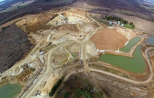
The fracking boom in the United States has created a voracious hunger for what’s known as “frac sand. It happens that there are huge deposits of just that kind of sand in Minnesota and Wisconsin. Result: the fracking rush in North Dakota has sparked a frac sand rush in the Upper Midwest. Thousands of acres of fields and forests have been stripped away so that miners can get their hands on those rare grains.
Thanks to the fracking boom, which kicked into high gear in 2008, the United States has overtaken Saudi Arabia and Russia to become the world’s biggest oil and gas producer. None of this could happen without sand. America’s fracking fields are the latest front to which we have deployed armies of sand to maintain our lifestyle.
By shooting a highly pressurized mix of water, chemicals, and sand into a well bore, drillers shatter the surrounding shale, spider-webbing it with tiny cracks through which the hydrocarbons can flow. They need the sand to keep the cracks open, holding fast against the pressure of the surrounding rock that wants to close them back up.
Every one of those wells needs sand, and lots of it. A single well can use as much as 25,000 tons—enough to fill more than two hundred railroad cars. But like members of a specialized combat unit, frac sand grains need to meet a list of highly specific physical requirements. They must be hard enough to withstand all that pressure, which means they must be at least 95 percent quartz.4 That eliminates most common construction sand, shrinking the pool to the silica sands used for glassmaking. But frac sand must also have the right shape: small enough to fit snugly into the frack cracks and rounded enough to let the hydrocarbons slide easily around them.
Most quartz grains, you’ll recall, are angular; there aren’t many places where you can find grains with such high purity and low angularity. The quartz sands under the ground of western and central Wisconsin have just that rare combination. These are ancient grains that were eroded, transported, then buried and uplifted again. Generally speaking, the older a grain is, the more rounded it is, thanks to however many extra million years of having its angles and edges worn down. Wisconsin also happens to have an excellent rail network and relatively lax environmental regulations. And so the fracking boom has sparked a frac-sand boom in the Badger State. Thousands of acres of the state’s farmland and forest are being torn up to get at the precious silica below.
In 2010, there were ten frac sand mines and processing plants in Wisconsin; four years later, that number had shot up to 135.6 The state produced around 25 million tons of frac sand in 2014, worth nearly $2 billion.
Production is likely to continue growing, since oil and gas operators have learned that increasing the amount of sand they shoot into a well increases the yield of oil or gas. New frac sand mines are also being opened in Texas as producers seek sources closer to the oil fields.
Nationwide, the legions of silica sand used for fracking have grown tenfold since 2003.7 They now dwarf those used for glassmaking and all other purposes, including silicon chips. By 2016, total silica sand production stood at nearly 92 million tons per year, almost three-quarters of which was used for fracking. Only 7 percent went to the glass industry.
The first step, he explained, is for excavating machines to scrape off the “overburden”—the plants, trees, topsoil, and unwanted miscellaneous rock lying on top of the sandstone that is their target. One reason Wisconsin silica sand is so desirable is because it lies very close to the surface, requiring relatively little digging to get at it.10 The topsoil is piled somewhere out of the way; it will be needed to help reclaim the land once the mine is tapped out, as required by law.
Once the sandstone is exposed, blasting experts drill a grid of holes into it, pack them with explosives, and simply blow a chunk of the hillside to smithereens. The sandstone shatters and collapses in a heap of . . . well, sand and stones. Front-end loaders dump the raw sand into trucks. After the “raw pile” is cleared away, excavators tear off another swatch of overburden and the process starts again, the hill disappearing slice by slice.
Down on the mine floor, the trucks haul the sand a few hundred yards to another pile, from where it’s fed into a complicated behemoth of a machine, a forty-foot-high Frankenstein of pipes, tanks, ladders, catwalks, and conveyor belts. A series of belts haul the sand up some thirty feet to a sorting screen, where jets spray it with water to turn it into a slurry. This sand-water mixture is then pumped onto a series of vibrating metal screens, which separate out first the miscellaneous rocks, then the oversize grains, shuffling these unwanted bits into a waste pile. Once everything bigger than .8 millimeters has been screened out, the remaining slurry is pumped up through corrugated pipe into a kind of upside-down pyramid called a hydrosizer. One hundred jets blast down into the cone, creating a carefully calibrated rising current that carries the lighter grains up and over the top into a trough, while the heavier ones sink to the bottom. By controlling the strength of the jets, you control the size of the grains that sink.
That sand is then run through a series of four attrition tanks—basically giant washing machines that spin the slurry, making the grains grind against one another, washing off silt or other impurities that might coat them. Last stop is a dewatering screen, a mesh of tiny slots measuring .01 millimeters, big enough for water to get through but not sand.
The sand is taken next to the drying plant, a vast warehouse-style building a few hundred yards away. Trucks load the washed sand into a metal hopper that feeds it onto another series of rising conveyor belts that carry it up to a doorway in the dryer plant, some twenty feet above the ground. Inside is a cavernous space, untouched by natural light, filled with another set of machines. The sand gets one more sifting, to filter out any stray rocks that might have gotten in on the journey from the pile, and then is fed through a long cylindrical tank.
A series of ducts underneath the tank blows hot air upward, drying the sand, while smokestack-like chimneys whisk away stray silica dust. “That’s the bad shit,” says Losinski. “That’s the stuff you don’t want to breathe.” Crystalline silica dust is sharp and jagged, especially when it’s freshly formed—like that found at sand mines and processing sites—and it can wreak havoc on the lungs. It’s been known for decades that too much exposure can cause silicosis, an especially severe lung disease.
A final relay of vibrating screens separates the sand into three size grades. Those are then hauled up a hundred feet in bucket elevators, vertical conveyor belts fitted with dozens of fiberglass buckets, and dumped into one of the 3,000-ton silos atop which Losinski and I stood. Trucks drive right up to the silos, fill up, and haul the product to the nearest rail station in Winona, Minnesota. From there, it’s off to the fracking fields.
There are a number of potentially serious risks to be concerned about. The first is water. The mines need lots of it to create their slurry and to wash the sand; a single mine can run through as much as 2 million gallons per day. The miners get a lot of it from high-capacity wells, which pump more than 70 gallons a minute from underground aquifers. “There’s a lot of concern about whether that will affect groundwater and trout streams fed by these headwaters
There’s also the question of what to do with wastewater that has been used to wash and process the sand. Typically the wastewater gets pumped into settling ponds; this is where the flocculants Pat Popple worries about are added in. Flocculants help remove particles suspended in the water, which is good. But they also contain acrylamide, a neurotoxin and carcinogen, which is bad.
That compound could potentially leach from the ponds into groundwater or surface water, warns a 2014 report
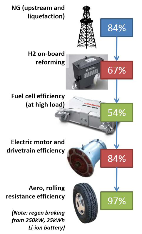
Figure 1. FCEV Heavy truck: PEM hydrogen fuel cell on-board reforming. U.S. Department of Energy Vehicle Technologies Program, Estimated for 2020. Source (DOE 2011).
Preface. There are 3 articles that I summarize below:
ARB. November 2015. Medium- and heavy-duty fuel cell electric vehicles. Air Resources Board, California Environmental Protection Agency.
NRC. 2003. Energy and Transportation: Challenges for the Chemical Sciences in the 21st Century. National Research Council
NACFE. 2020. Making sense of heavy-duty hydrogen fuel cell tractors. North American council for freight efficiency. It has additional information in hydrogen fuel cell (FCEV) trucks.
Figure 1 reveals why hydrogen fuel cell trucks are incredibly inefficient. Turning hydrogen back into electricity with a fuel cell is only 24.7 % efficient (.84 * .67 * .54 * .84 * .97) as shown in figure 1. There are multiple stages where energy is lost due to inefficiencies at each step: Natural gas upstream and liquefaction, hydrogen on-board reforming, fuel cell efficiency, electric motor and drive-train losses, and aerodynamic/rolling resistance.
Since fuel cell electric trucks are terrible at acceleration, they always have a second propulsion system, usually a battery, making them orders of magnitude more expensive than an equivalent diesel truck, $1,300,000 versus $100,000 respectively.
Hydrogen is not a renewable, since 96 to 99% of hydrogen is made from natural gas using natural gas, but at least it can be made cheaply around the clock that way.
Hydrogen generated with solar power could only be made 10 to 25% of the time (the capacity factor) when the sun is up, and electrolysis of water is so expensive it is only made for applications that require extremely pure hydrogen, mainly NASA. The amount of space rebuildable contraptions like solar and wind take up is a problem as well. To use wind power to produce 700 Terrawatt hours of hydrogen would require wind turbines taking up 40,154 square miles (Ford 2020).
Hydrogen pipelines are too expensive to build at length, since they are corroded and embrittled by hydrogen. Yet delivery would require a $250,000 canister truck weighing 88,000 pounds (40,000 kg) delivering a paltry 880 (400 kg) of fuel, enough for 60 cars and just a few trucks. A diesel truck can carry 10,000 gallons of gas, enough to fill 800 cars. The hydrogen delivery truck cannibalize much of its energy: over a distance of 150 miles, it will burn the equivalent of 20% of the usable energy in the hydrogen it is delivering (Romm 2005).
Trucks don’t use hydrogen tanks because they take up 10% of payload weight (DOE 2011), or fuel cells, because the best only last 2500 hours but need to keep on going at least 14,560 hours in long-haul trucks and 10,400 in distribution trucks (den Boer 2013).
The few FCEV that exist are heavily subsidized by agencies like the California Air Resources Board Hybrid & Zero emission truck voucher incentive program (HVIP) of up to $288,000 per truck (CASEY 2023)
ARB. November 2015. Medium- and heavy-duty fuel cell electric vehicles. Air Resources Board, California Environmental Protection Agency.
Medium- and heavy-duty Fuel Cell Electric Vehicles (FCEV) are far from being commercial due to many barriers:
Vehicle cost (bus): $1,300,000
Vehicle cost (truck): even higher due to heavier payloads
Cost of hydrogen fuel
Cost of fuel cell power plant. At $3,000/kW for a 150 kW fuel cell system, the power plant cost is $450,000
Cost of 40-50 kg fuel tank, frame, and mounting system is $100,000
Service station costs of $5,000,000 and O&M costs of $200,000/year
Distribution of hydrogen fuel (corrodes pipes, distributed by diesel-burning trucks now)
More frequent fueling (the fueling infrastructure for FCEV medium and heavy-duty trucks is not known since there aren’t any commercial MD/HD trucks yet)
Lack of hydrogen service stations
Significantly higher costs for FCEV than diesel trucks
Hydrogen tanks weigh a lot
Hydrogen tanks take up a lot of space
Tank weight and size reduce range
Hydrogen is more expensive than diesel fuel
The only public hydrogen stations in California are for light duty cars. Because of the high pressure at which they dispense hydrogen, as well as different fueling protocols and nozzles, they are not compatible for use with current fueling protocols for medium- or heavy-duty vehicles.
FCEV can’t handle acceleration well so there is always a 2nd propulsion system like batteries, which adds to their cost
Tanks can go on the roof of buses, but trucks do not have enough space for a tank (though there is room for the fuel cell which is roughly equal to a conventional diesel engine with a similar power rating)
Only PEM fuel cells with low operating temperatures, high power density, and so on are suitable, but they are too fragile to endure the rough ride of a truck
FCEV use too much platinum metal group elements which are limited and expensive
What is an FCEV? A FCEV is a vehicle with a fuel cell system that generates electricity to propel the vehicle and to power auxiliary equipment. Hydrogen fuel is consumed in the fuel cell stack to produce electricity, heat, and water vapor—no harmful pollutants are emitted from the vehicle. FCEVs are typically configured in a series hybrid design where the fuel cell is paired with a battery storage system. Together, the fuel cell and battery systems work to meet performance, range, efficiency, and other vehicle manufacturer goals. FCEVs have higher efficiencies, quieter operation, comparable range between fill-up, and similar performance to conventional vehicles.
Most suitable applications. Vehicles that are centrally fueled, operated, and maintained, returning to the same base at the end of the day.
NRC. 2003. Energy and Transportation: Challenges for the Chemical Sciences in the 21st Century. National Research Council
Excerpts about hydrogen fuel cells:
The most important part of a fuel cell is the membrane, which must be an ion conductor, an electronic insulator, an impermeable gas barrier and also possess good mechanical strength. However, the key issues in making a practical fuel cell are non-electrochemical. These include the acts of delivering the gases to the fuel cell membrane, removing the water, removing the heat from around the system, and controlling humidity and pressurization of gases. There are still many challenges for electrochemists, chemists, and chemical engineers. For example, a membrane that is more tolerant of environmental conditions for gases of varying pressures will allow for the elimination of various system components, which can be very expensive due to their use of stainless steel. The technical challenge is in fabricating a membrane to be thin enough so that the hydrogen side of the gas supply does not need to be humidified. However, as membranes get thinner, reliability over long periods of time becomes an issue due to faradaic losses. If the membrane is too thick, additional components must be added to humidify the hydrogen.
In a vehicle fuel cell stack, which has over 400 cells in series, the situation is even more complicated. Well over 90% of fuel cell industry funds are not spent on the membrane but on moving these gases in and out of the fuel cell stack, managing the system, and creating the environment where the membrane can do its job. Fuel cell research, however, is mainly performed in a lab where gases are supplied at exactly the right humidity, pressures, and so on. The actual commercial problem, development of a fuel-cell-powered vehicle that has a life of 15 years and 150,000 miles under terrible external environmental conditions, has not been approached.
Tolerances are also not well understood. A fuel cell stack with over 400 cells operating in this environment contains sealant, which is literally miles long. Seals will start to fail after the fuel cell is bumped and jostled on the highway and while temperature shifts between hot and cold, and the cell is turned off and on. With zero tolerance for safety failures, hydrogen leaks cannot occur with these vehicles. Additionally, every cell has to be identical or the system cannot be managed. Unfortunately, that kind of tolerance control is not yet available.
An ideal fuel cell system will have minimal components outside of the stack and will operate using ambient, unhumidified hydrogen. Although fuel cells are very efficient, they do not release much heat through the exhaust. Even though they generate less heat than an internal combustion engine, the system requires the addition of cooling components due to the generated heat in the cooling stack. However, if this stack can generate less heat, then radiators, pumps, and coolant will not be required.
The standard for a modern vehicle requires it to start within 2 seconds at worst. A fuel cell starts well within 1 second. However, fuel cells, including hydrogen fuel cells, do not operate well at subfreezing temperatures. This is because fuel cells are basically a liquid interface device and need liquid-phase water to operate. Running the system under the conditions of a highway environment is possible, but the current cost is too great for commercialization.
Practical use of hydrogen in vehicles may never happen until there is a better method to store hydrogen, especially since onboard reforming of hydrogen at a reasonable cost may not be a possibility.
The use of hydrogen requires additional infrastructure for production and transportation. One method is to use electrical energy to produce hydrogen, but power grids are very inefficient. Another is the use of a natural gas pipeline, which is also wasteful since it involves the liquefying and re-evaporation of gases.
End note: Sir William Robert Grove invented the hydrogen fuel cell or “gas battery” in the 1840s. The first practical fuel cells were not built until the Gemini and Apollo space programs in the 1960s and are still used in space today. The difference between building a successful fuel cell and a commercially successful fuel cell, however, is the same difference between putting a man on the moon and putting 10,000 men on the moon every day at an affordable price. We’re running out of time to invent a good hydrogen fuel cell, they’ve been around 180 years, and peak oil may have occurred in 2018 (Patterson 2019).
NACFE. 2020. Making sense of heavy-duty hydrogen fuel cell tractors. North American council for freight efficiency.
A few bits and pieces from this document.
Currently there are less than 8,573 hydrogen fuel cars, 48 buses, and 20 prototype trucks, most of them in California, where there are 15 retail hydrogen stations.
Estimates of an electric future with both battery electric and fuel cell vehicles will need anywhere from 2X to 8X the amount of electric energy produced today. Similarly, little of today’s hydrogen production is used for transportation. The production of both electricity and hydrogen will need to aggressively increase; and in lockstep, the demand for both will need to dramatically increase.
Today there are only a handful of prototype fuel cell demonstrator trucks in existence, each built to be successful for certain applications. Since there are only pilot vehicles, mainly in Switzerland, this report can’t say much about how they operate in real life. The costs of hydrogen, vehicles, and hydrogen production all must come down significantly to make hydrogen economically competitive with alternatives.
In order for trucks to use hydrogen, all of the following must be in place: H2 production plants need to be built and produce H with economies of scale 2) There has to be a demand for H (market penetration), 3) A distribution network must exist from production facilities to end users, 4) The delivery technology to quickly deliver high pressure H fuel in volume needs to be developed 5) Storage technology to safely and efficiently store hydrogen for distribution, fueling, and onboard the vehicle in place 6) H technology must be reliable, 7) Cheap electricity is required for electrolysis, 8) Battery cell costs must come down and energy density increase, 8) H must be safe and technicians, drivers, and emergency personnel trained to deal with problems 9) The Green H must be sustainable, available, and affordable
Quickly ramping up both electricity supply and demand, in the matter of a couple decades or less, is challenging. Application of funding can only do so much. Innovations will be required across a range of technologies.
Hydrogen colors
Green: electrolysis of water with electricity from renewable resources. Zero carbon emissions
Turquoise: thermal splitting of natural gas, instead of CO2 solid carbon produced
Pink / purple / red: produced by nuclear power electrolysis
Black / gray: from natural gas using steam-methane reforming
Yellow: electrolysis with grid electricity
Brown: from fossil fuels, usually coal, with gasification
Blue: gray or brown with CO2 sequestered or repurposed
White: byproduct of industrial processes
The truck manufacturing marketplace is entirely about supply and demand. The annual trucking market demand for new vehicles and the annual trucking manufacturing output range from 150,000 to 300,000 vehicles per year. In 2020 there were zero Class 8 fuel cell trucks produced.
In 2030, 30% of new Class 8 vehicles would optimistically be approximately 100,000 vehicles a year. There are an estimated 1.8 million Class 8 trucks hauling freight trailers in the United States today. In total, there may be up to 4 million Class 8 vehicles registered in the United States with the lives of those vehicles ranging from 12 to 20 years or more.
Trucks are long-term capital investment tools. Commercial vehicle populations change slowly. The vehicles have long life spans. It can take 20 years or more for a new technology to completely supplant an existing one through normal market attrition.
Hydrogen fuel cell trucks can be superior to Battery electric trucks if
Zero emission at tailpipe important
Tractor tare weight critical to maximizing payload
Long distance routes over 500 miles common
Winter conditions significant
Green or blue H available
Incentivized Hydrogen use
Less mountainous
As Steve Hanley of CleanTechnica summarized, “Making electricity to electrolyze hydrogen which is then used in fuel cells to power vehicles is not as efficient as making electricity and using it to power vehicles directly in the first place. Every time energy gets converted from one form to another, there are losses. The more transformations there are, the more losses occur.”
How do Heavy-duty Hydrogen Fuel Cell tractors (FCEV) vehicles work?
In all cases, FCEV also need to have batteries.
A battery dominant FCEV uses the fuel cell to charge the onboard batteries. The batteries then directly power the electric motors. As the batteries deplete running the motors, the fuel cell provides some replacement of energy, but the battery dominant system expects that the duty cycle will reduce the state of charge (SOC). Sized correctly for the duty cycle, the vehicle ends it shift before the battery SOC is completely depleted. Complete depletion generally means some low SOC cutoff typically around 20% SOC [3]. The fuel cell then recharges the parked truck prior to its next shift.
A fuel cell dominant vehicle will use both the fuel cell and the battery pack to power the electric motors. The battery pack serves to handle short demand peaks, like accelerations or short hills, while the fuel cell is sized to provide continuous power to the motors for a typical average duty cycle load. There is a balance between planned typical loads and peak loads that dictates how much battery and how much fuel cell is required for the expected duty cycles. Designers need to statistically predict nominal and off-nominal loads to properly size the systems for the end user. A dedicated route with predictable freight loads and repeatable traffic and weather conditions can allow smaller battery packs for a fuel cell dominant system. Variable routing with a wide variety of payloads and complex traffic and weather conditions may require a more battery dominant system with greater battery capacity to compensate for the unpredictable duty cycles. Conversely, this variable route also might be served by having larger fuel cell(s) rather than battery packs
Hydrogen tanks
While spherical hydrogen tanks are the optimum for the weight-to-strength ratio, they do not package well on trucks. Long, constant diameter cylinders with rounded ends are the primary shape to consider. These shapes are very similar to those evolved for CNG-based trucks where they are typically packaged behind the cab in modular units. Placing the tanks behind the cab increases the wheelbase. Placing the tanks in this region also requires maintaining adequate swing and dip clearances to trailers, so trailer gaps need to be maintained.
Ballard said, “Using an estimated specific density of 36kg tank weight per 1kg of hydrogen yielded a tank weight of 3910kg (8,600 lbs.)” in its report on the potential of applying fuel cells to NACFE’s Run on Less Regional demonstration fleet diesel vehicles. The net weight impact was estimated by Ballard “to weigh 7,750 lbs. (3,520kg) more than a diesel truck.” A gauge for estimating relative weight impact of fuel cell tractors is that current CNG trucks are approximately 1,500-2,000 lbs. heavier than their diesel counterparts, the added weight due to the net impact of the tanks, plumbing and frame length versus the parts removed from emission systems. The current prototype battery electric drayage trucks are approximately 7,000 to 10,000 lbs. heavier than diesel, NACFE learned from consultations with a variety of sources operating these early prototype vehicles. Fuel cell tanks will be somewhat heavier than their CNG counterparts in order to deal with the higher pressures.
Carbon fiber has become a material of choice to use in hydrogen tanks for vehicles. Carbon fiber has the strength of steels yet is 10%-30% lighter for the same performance. They can be three to five times more energy intensive to fabricate than conventional steel, according to the DOE group that evaluates and promotes lightweight material manufacturing and use, the Advanced Manufacturing Office (AMO). There are cost increases with using carbon fiber over steel, as lightweight materials generally carry cost premiums since they are more expensive in energy, time and effort to make.
Fuel Cell buses
There are 14 operating today, with an average cost of $1,920,000 ($1,270,000 to $2,400,000). They are not yet at the commercial stage, but in the technology demonstration state. Class 8 trucks are significantly more demanding than buses, which will require many years of development to reach the commercial stage. heavy-duty trucks see 80,000 miles to more than 140,000 miles per year pulling heavy loads in all weather and traffic conditions. Where buses have known dedicated routes and conditions, with generally slower speeds and passenger friendly stopping and accelerations, heavy-duty trucks see highway speeds and urban travel with more demanding stops and starts due to their 60,000- to 80,000- lb. vehicle weights. It’s not that automotive and bus technology cannot migrate to trucks, but the systems that do migrate must go through significantly greater validation to achieve reliability, environmental and performance requirements as outlined in NACFE’s Defining Production report [33].
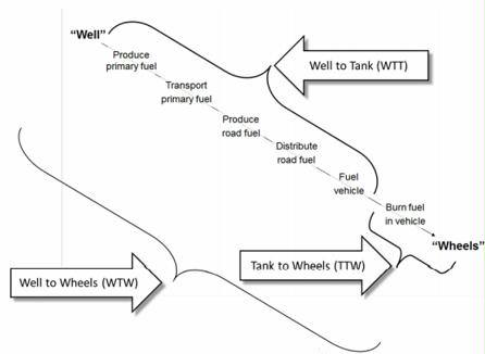
Efficiency: While the vehicle fuel efficiency is an important indicator, a whole system perspective is also needed — what is termed well-to-wheel (WTW) as opposed to tank-to-wheel (TTW) or well-to-tank (WTT)
Well to wheel (WTS) versus tank-to-wheel (TTW) and well-to-tank (WTT)
WTW quantifies the entire system from extracting oil in the ground, to transporting it to a refinery, to refining it into diesel fuel, to transporting the diesel fuel to a truck stop, storing it and ultimately delivering the fuel into a truck’s fuel tank, and then finally consuming the fuel to move the truck down the road. Efficiencies for the total system are much more challenging to measure because details of all intermediate steps are not always visible and quantifying them through prorating can be complex.
From a public policy perspective, the real killer for H2FC cars is their wind-to-wheel (or solar-to-wheel) inefficiency. Driving a small family car 100km, whether H2FC or BEV, uses 15kWh of motive energy at the wheels. For the BEV, taking into account losses on the grid and in the battery cycle and drive train, that translates into a need to generate 25kWh at the plant where the electricity is generated. The equivalent for the H2FC car, given losses in electrolysis, compression, transport, storage and reconversion of hydrogen, is at least 50kWh. Put simply, hydrogen cars are half as efficient as BEVs – and there is no reason in physics to think that will change. There is reason why [Teslas’s] Elon Musk calls them “fool cell” cars. BEVs are 2X to 3X more efficient than hydrogen fuel cells on a WTW basis
Safety
Hydrogen-based tractors may not be viable for all routes in the U.S. or Canada due to unacceptable levels of risk in locations such as the Eisenhower Tunnel in Colorado or other tunnels and enclosed spaces like warehouses or underground facilities. The challenge is that transporting highly combustible fuels is sometimes restricted on routes. Fuel haulers have additional rules to follow. A hydrogen fuel cell truck is hauling not only a highly combustible fuel, it is hauling a 10,000 psi storage container. A further modern element of concern is intentional use of these vehicles as weapons in terrorism. This risk is likely similar to that faced by fuel haulers, which may necessitate additional driver certification and background checks for hydrogen powered tractors.
Emissions
Adding to the complexity of defining the system is that physically making the vehicle and the infrastructure to support it also factors into the net system emissions. For example, while a wind turbine spinning in Texas is emission free in providing energy, prior to that point, fabricating, shipping and installing the wind turbine blades and parts are not emission free, and typically require fossil fuel energy expenditures to get the raw materials and then to manufacture (under business as usual). These wind turbines are capital investments which wear out in use, and parts must be disposed of, again requiring energy expenditures and having environmental considerations.
Calstart. 2013. I-710 project zero-emission truck commercialization study. Calstart for Los Angeles County Metropolitan Transportation Authority. 4.7.
Casey T (2023) For Fuel Cell Trucks, Nikola Cooks Up Hydrogen Fueling Station On-The-Go. https://cleantechnica.com/2023/01/28/for-fuel-cell-trucks-nikola-cooks-up-hydrogen-fueling-station-on-the-go/
den Boer, E. et al. 2013. Zero emissions trucks. Delft.
DOE. 2011. Advanced technologies for high efficiency clean vehicles. Vehicle Technologies Program. Washington DC: United States Department of Energy.
Ford, J. 2020. The world must look beyond sun snd wind for hydrogen. We need lots of the gas, and cheaply, if it is to help replace liquid carbon fuels. Financial times
ICCT. July 2013. Zero emissions trucks. An overview of state-of-the-art technologies and their potential. International Council for Clean Transportation.
Preface. The article below argues that electric cars aren’t going to replace gas and diesel vehicles enough to lessen greenhouse emissions.
The average electric vehicle requires 30 kilowatt-hours to travel 100 miles — the same amount of electricity an average American home uses each day to run appliances, computers, lights and heating and air conditioning. If electric cars expand, a U.S. Department of Energy study found that increased electrification across all sectors of the economy could boost national consumption of electricity by as much as 38% by 2050, in large part because of electric vehicles (Brown 2020).
I would argue that since two-thirds of electricity is still generated with natural gas and coal, emissions will certainly go up. Wind and solar won’t put much of a dent in that 66% fossil usage in the future either, because the best areas for solar and wind power have already been built, and the new transmission lines cost far more than the solar and wind power generated in more distant unexploited areas. Also, when natural gas and coal are burned to generate electricity, two-thirds of the energy contained in them is lost as heat, so only one-third of their energy makes it onto the transmission grid, where another 6 to 10% is lost over the wires, so as little as 23% of the fossil energy reaches your electric socket. Better to just burn the natural gas directly in cars perhaps.
And finally, until we have massive energy stored in batteries and pumped hydropower, we simply have to have natural gas to balance intermittent wind and solar power or they’ll bring the grid down.
Do the math: expensive electric cars that only the top 5% can afford are not replacing natural gas and coal.
The number of automobiles on the world’s roads is on pace to double — to more than two billion — by 2030. And more likely than not, most of those cars will be burning carbon-emitting gasoline or diesel fuels.
That is because much of the expansion will be propelled by the rise of the consumer class in industrializing parts of the globe, especially in China and India, as hundreds of millions of new drivers discover the glory of the open road. Those populous and geographically sprawling countries might be hard pressed any time soon to assemble the ubiquitous electricity grid required for recharging electric vehicles; and much of the electricity China and India will produce in coming decades will come from coal-fired power plants that are some of the planet’s biggest emitters of carbon dioxide.
Given the limitations of electric cars so far — including their limited range between charges — many experts predict that most of the billion additional cars predicted to be on the road in 2030 will have internal combustion engines that spew greenhouse gases.
But virtually everyone who studies the issue understands that transportation, which is still 95% reliant on petroleum, is the world’s fastest-growing energy-based contributor to greenhouse gases. About three-quarters of the total comes from motor vehicles.
But optimists argue that even in the case of cars with internal-combustion engines, carbon dioxide emissions can be cut significantly by measures like increasing fuel economy and introducing smart-driving technologies to make cars move about with greater efficiency.
The countries with the most cars today have set aggressive goals for improving fuel mileage. The United States, under President Obama’s fleetwide standards for carmakers, is aiming for an average of 54.5 miles per gallon by 2025, up from about 30 m.p.g. now. China is aiming for 50.1 miles per gallon, and the European Union 60.6.
Still, the math is daunting. If the number of cars doubles, and the average mileage improves by only 50%, all of the fuel-economy gains would be offset by the emissions from the new vehicles.
And that assumes the auto industry does its part to comply with the new standards and that national regulators diligently enforce them. Recent revelations that Volkswagen, for one, deliberately misled regulators, and that European Union air-quality standards and enforcement have been far from rigorous, do not inspire confidence.
“But the automakers are attacking these standards as we speak, both in Congress and through a review of the program they demanded from the Obama administration,” Mr. Becker said. “Similar attacks are underway in the E.U.”
Congress, in an effort to make the United States more energy independent, passed a law in 2007 mandating a 35 m.p.g. auto-fleet standard by 2020. But before that, there had been no official change to American fuel-economy standards in more than 30 years.
“The U.S. auto industry was successful between 1975 and 2007 in preventing any improvement for mileage standards for CO2 emissions,” Mr. Becker said. “They exploit every loophole in the standards, making more SUVs, pickups and other light duty trucks than cars because trucks have weaker standards than cars, and more large vehicles because large vehicles have weaker standards than smaller vehicles.”
But Mr. Becker, at the Safe Climate Campaign, points out that electric vehicles are only as environmentally friendly as the electricity that recharges them. China, though it is rapidly adopting nuclear power plants, is still heavily reliant on coal-fired electrical plants.
And India, where the biggest growth in automobile ownership is expected to occur as the country industrializes and its population surpasses China’s by 2030, might actually increase its reliance on coal-fired electrical power plants between now and then.
“At the end of the day, when you talk about transport emissions for transport in general, including for freight transport, they increase when the economy is growing,” he said. “So what are we going to say, we’re going to stop the economy to stop emissions?”
Preface. The four articles below explain why methane from permafrost or hydrates are not likely to erupt abruptly and send Earth into a hothouse hell. In addition, here are some posts debunking Guy McPherson who believes the world will end in a methane apocalypse:
Researchers studied methane emissions from a period in Earth’s history partly analogous to the warming of Earth today. Their research, published in Science, indicates that even if methane is released from these large natural stores in response to warming, very little actually reaches the atmosphere in large quantities.
This finding suggests that methane emissions from future warming will likely not be as large as some have suggested.
This is due to several natural buffers. In the case of methane hydrates, if the methane is released in the deep ocean, most of it is dissolved and oxidized by ocean microbes before it ever reaches the atmosphere.
If the methane in permafrost forms deep enough in the soil, it may be oxidized by bacteria that eat the methane, or the carbon in the permafrost may never turn into methane and may instead be released as carbon dioxide.
A popular theory of a giant methane burp as the killer is known as the “clathrate gun” hypothesis posits a sudden and massive release of methane hydrates from the land, on ocean shelves, and the depths of the ocean. There are many reasons to question this though:
Majorowicz (2014) found methane hydrate reservoirs would have melted over 100 to 400 thousand years in the hothouse Permian world, long before the first extinction pulse
Hydrates only form in cool oceans, like those of today, and there isn’t much carbon in them, somewhere between 500 and 2500 GtC (Milkov 2004). Yet this is far more than what would have existed in Permian oceans, and just a small fraction of the overall 24,000 to 46,000 GtC Siberian Trap emissions.
Ocean hydrates would have also been far less extensive than they are today because super continent Pangea had far fewer miles of hydrate-containing continental shelves than the shelf length of our multiple continents today (Wignall 2017).
Methane is a far more powerful greenhouse gas than carbon dioxide, but doesn’t last long in the air because it oxidizes to CO2 and water vapor in about 9 years
It is not likely deep water methane hydrates would reach the atmosphere since they’d be oxidized in the water column (Rupple 2011).
Even if there were a methane hydrate burp in the first killer pulse, a new suspect has to be found for the second killing pulse, since there was no cooling in the 200,000 year interval between them. It takes millions of years of cold water for methane hydrates to form again after they’ve melted.
Milkov (2004) concludes “A significantly smaller global gas hydrate inventory implies that the role of gas hydrates in the global carbon cycle may not be as significant as speculated previously.
References
Majorowicz, J., et al. 2014. Gas hydrate contribution to Late Permian global warming. Earth and Planetary Science Letters 393:243-253.
Milkov, A. 2004. Global estimates of hydrate-bound gas in marine sediments: How much is really out there? Earth-Science Reviews 66: 183-197.
Rupple, C. D. 2011. Methane Hydrates and Contemporary Climate Change. Nature Education Knowledge.
Wignall, P. B. 2017. The Worst of Times: How Life on Earth Survived Eighty Million Years of Extinctions. Princeton University Press.
Recent studies (e.g. Whiteman et al) have raised the alarm that methane emissions could occur in the Arctic, especially over the East Siberian Shelf and in Siberian Lakes (e.g. Shakhova et al). However, there is a vigorous academic debate on the origin and potential impact of these emissions. As acknowledged by the IPCC: “How much of this CH4 originates from decomposing organic carbon or from destabilizing hydrates is not known. There is also no evidence available to determine whether these sources have been stimulated by recent regional warming, or whether they have always existed since the last deglaciation. More research is therefore urgently needed.
The first uncertainty is the amount of gas hydrates stored on Earth. Global gas-in-place estimates range over an order of magnitude 1,000-20,000 tcm, with most estimates around 3,000 tcm. Estimates are even more uncertain at the regional level. For instance, there are no models for Antarctic reservoirs, and estimates for Arctic permafrost have only been done recently.
In the permafrost, additional uncertainty arises from the origin of methane emissions, whereas in the case of ocean sediments, the mechanisms by which methane is released and its ability to reach the atmosphere are also disputed. So are the biochemical and chemical consequences that gas-hydrate releases would have on oxidation mechanisms e.g. there may be resource limitations hindering methane oxidation in the ocean.
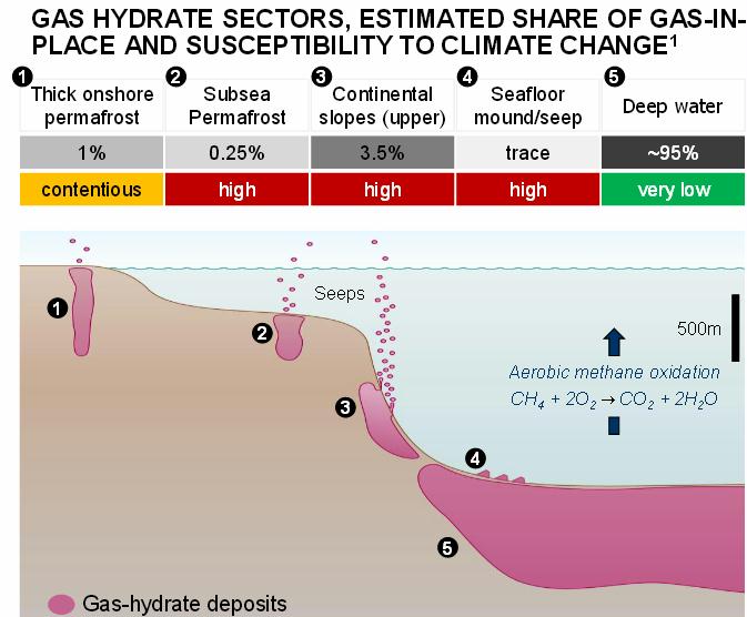
Since gas hydrates are only stable under high pressures and at low temperatures, there have been concerns that climate change could result in gas-hydrate dissociation and the release of methane into the atmosphere. The response of gas hydrates to climate change has only been investigated recently. Modelling in this field is in its infancy and faces major uncertainties. Nevertheless, it is generally agreed that gas-hydrate dissociation is likely to be a regional phenomenon, rather than a global one, and more likely to occur in subsea permafrost and upper continental shelves than in deep-water reservoirs, which make up the majority of gas hydrates. Indeed,the later are relatively well insulated from climate change because of the slow propagation of warming and the long ventilation time of the ocean. Moreover, the release of methane from gas-hydrate dissociation should be chronic rather than explosive, as was once assumed;and emissions to the atmosphere caused by hydrate dissociation should be in the form of CO2 because of the oxidation of methane in the water column.
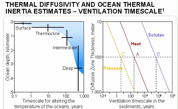
Graphs adapted from Archer (2007), “Methane hydrate stability and anthropogenic climate change”. In the graph on the right, ventilation timescale corresponds to the timescale required by temperature (heat), pressure and solutes such as methane to diffuse through the sediments
Ocean thermal response varies according to depth, as highlighted in the graph above (left), but also from place to place, especially in deep-water locations, due to ocean currents. In sediments, the diffusion of heat towards deeper layers takes time and varies primarily according to depth, but also according to the composition of the sediment and to the geothermal gradient. Heat can diffuse approximately 100 meters in about 300 years (point A). Solutes such as dissolved methane diffuse even more slowly (100 meters in about 30,000 years), point B), while pressure perturbation (e.g. following a sea-level rise) diffuses more quickly (100 meters in about 3 years), point C.
As a result of thermal inertia, heat diffusion and the melting of permafrost take time, and should be slow enough to insulate most hydrate deposits from expected anthropogenic warming over a 100-year timescale. Nevertheless, temperature increases in high latitudes, such as the Arctic, are expected to be much higher than increases in the mean global temperature, and are therefore more likely to affect gas-hydrates reservoirs. Rises in sea level would result in pressure increases at the seafloor that may mitigate further dissociation of offshore gas-hydrate deposits. However, it is likely to be insufficient to negate the warming.
Even if warming were to reach the gas hydrate stability zone, the fate of any methane released would be uncertain.Gas could escape if the pressure exceeded the sediment’s lithostatic pressure, but it might also remain in place. In addition, since gas-hydrate dissociation will start at the edge of the stability zone, even if gas were able to migrate, it might subsequently be trapped in newly formed hydrates.
Finally, even if methane were able to migrate towards the seafloor, it would probably not reach the atmosphere. Most methane is expected to be oxidized in the water column rather than released by bubble plumes or other “transport pathways” directly into the atmosphere as methane. Nevertheless, the oxidation of methane produces CO2, which will have an impact on ocean acidification and will remain in the atmosphere.
The susceptibility of gas-hydrate deposits to climate-change-induced dissociation varies significantly, according to reservoir location. (1) Moridis et al.2011. Challenges, uncertainties and issues facing production from gas hydrate deposits.
The risk of climate change causing gas-hydrate dissociation and methane leaks varies significantly by location.This can be explained by depth differentials, the existence of mitigation mechanisms such as water-column oxidation, or by the exposure of gas-hydrate deposits to varying regional warming phenomena. High-latitude warming is expected to be much greater than global-mean-temperature warming.
As a rule-of-thumb, gas hydrates held within subsea permafrost on the circum-Arctic ocean shelves and on upper continental slopes are the most prone to dissociation. Subsea permafrost, which were flooded under relatively warm waters due to sea level rises thousands of years ago, have been exposed to dramatic rises in temperature that have led to a significant degradation both of subsea permafrost and t he gas hydrates within it.The latter are believed to store a greater quantity of gas hydrates than the former, but methane releases are less likely to reach directly the atmosphere because of oxidation in the water column.
However, it is very unlikely that climate warming will disturb gas-hydrate deposits that are held in deep-water reservoirs around 95% of all deposits on a millennial timescale. Finally,
gas hydrates in seafloor mounds may also dissociate as a result of warming, overlying water or pressure perturbation, but these account for a very limited share of gas hydrates in place.
The sensitivity of gas-hydrate deposits in onshore permafrost,especially at the top of the hydrate stability zone, is more uncertain and subject to greater debate
Archer et al. calculated that between 35 and 940 GtC of methane could escape as a result of global warming of 3° C, with maximum consequences of adding a further 0.5° C to global warming. On top of the uncertainty reflected in the range above, there are other considerable uncertainties, notably concerning the effectiveness of mitigation mechanisms and the long-term outlook, since methane will continue to be released, even if warming stops.
Reagan and Moridis (2007), “Oceanic gas hydrate instability and dissociation under climate change scenarios”;
Maslin et al. (2010), “Gas hydrates: past and future geohazard?”;
Shakhova et al. (2010), “Predicted Methane Emission on the East Siberian Shelf”;
Whitemann et al. (2013), “Climate science: Vast costs of Arctic change”
Do the huge craters pockmarking Siberia herald a release of underground methane that could exceed our worst climate change fears? They look like massive bomb craters. So far 7 of these gaping chasms have been discovered in Siberia, apparently caused by pockets of methane exploding out of the melting permafrost. Has the Arctic methane time bomb begun to detonate in a more literal way than anyone imagined?
The “methane time bomb” is the popular shorthand for the idea that the thawing of the Arctic could at any moment trigger the sudden release of massive amounts of the potent greenhouse gas methane, rapidly accelerating the warming of the planet. Some refer to it in more dramatic terms: the Arctic methane catastrophe or methane apocalypse.
Some scientists have been issuing dire warnings about this. There is even an Arctic Methane Emergency Group. Others, though, think that while we are on course for catastrophic warming, the one thing we don’t need to worry about is the so-called methane time bomb. The possibility of an imminent release massive enough to accelerate warming can be ruled out, they say. So who is right?
Few scientists think there is any chance of limiting warming to 2 °C, even though many still publicly support this goal. Our carbon dioxide emissions are the main cause of the warming, but methane is a significant player.
Methane is a highly potent greenhouse gas – causing 86 times as much warming per molecule as CO2 over a 20-year period. Fortunately, there’s very little of it in the atmosphere. Before humans arrived on the scene there was less than 1000 parts per billion. Levels started rising very slowly around 5000 years ago, possibly to due to rice farming. They’ve gone up more since the industrial age began: the fossil fuel industry is by far the single biggest source, followed by farting farm animals, leaking landfills and so on. Only a tiny percentage comes from melting Arctic permafrost.
The level in the atmosphere is now nearing 1900 ppb, but that’s still low. CO2 levels were much higher to start with, around 270,000 ppb before the industrial age. They have now shot up to 400,000 ppb today. The main reason is that CO2 persists for hundreds of years, so even small increases in emissions lead to its buildup in the atmosphere, just as water dripping into a bath with the plug left in can fill the bath eventually.
Methane, by contrast, breaks down after just 12 years, so its level in the atmosphere can only increase if there are big ongoing emissions.
So for methane to cause a big jump in global warming there not only has to be a massive source, it has to be released very rapidly. Is there such a source?
Yes, claim a few scientists. They point to the Arctic permafrost, and specifically to the East Siberian Arctic shelf. This vast submerged shelf underlies a huge area of the Arctic Ocean, which is less than 100 meters deep in most places. During past ice ages, when sea level dropped 120 meters, the land froze solid.
This permafrost was covered by rising seas as the ice age ended around 15,000 years ago. The upper layer has been slowly melting as the relative warmth of the seawater penetrates down. But the frozen layer is still hundreds of meters thick. No one doubts that there is plenty of carbon locked away in and under it. The questions are, how much is there, how much will come out in the form of methane, and how fast?
Natalia Shakhova of the International Arctic Research Center at the University of Alaska Fairbanks, has been studying the East Siberian Arctic shelf for more than two decades. Her team has made more than 30 expeditions to the region, in winter and in summer, collected thousands of water samples and tons of seabed cores during four drilling campaigns and made millions of measurements of ambient levels of methane in the air.
Her team has estimated that there is a whopping 1750 gigatons of methane buried in and below the subsea permafrost, some of it in the form of methane hydrates – an ice-like substance that forms when methane and water combine under the right temperature and pressure. What’s more, they say that the permafrost is already beginning to thaw in places. “Our results show that… [the] subsea permafrost is perforating and opening gas migration paths for methane from the seabed to be released to the water column,” says Shakhova.
Her team’s work hit the headlines in 2010, when in a letter in the journal Science they reported finding more than 100 hot spots where methane was bubbling out from the seabed. But as others pointed out, it was not clear whether these emissions were something new or had been going on for thousands of years.
More sensational stuff was to follow. In another 2010 paper, the team explored the consequences of 50 gigatons of methane – 3% of their estimated total – entering the atmosphere (Doklady Earth Sciences, vol 430, p 190). If this happened over five years methane levels could soar to 20,000 ppb, albeit briefly. Using a simple model, the team calculated that if the world was on course to warm 2 °C by 2100, the extra methane would lead to additional warming of 1.3 °C, so temperatures would hit 3.3 °C by 2100.
This study appeared in an obscure journal and did not get much attention at the time. But then Peter Wadhams of the University of Cambridge and colleagues decided to see how much difference a huge methane release between 2015 and 2025 would make when added to an existing model of the economic costs of global warming. “A 50-gigaton reservoir of methane, stored in the form of hydrates, exists on the East Siberian Arctic shelf,” they stated in Nature, citing Shakhova’s paper as evidence. “It is likely to be emitted as the seabed warms, either steadily over 50 years or suddenly. Understandably, this was big news.
But in reality the idea that 50 gigatons could suddenly be released, or that there’s a store of 1750 gigatons in total, is very far from being accepted fact. On the contrary, Patrick Crill, a biogeochemist at Stockholm University in Sweden who studies methane release from the Arctic, says it is simply untenable. He wants Shakhova’s team to be more open about how they came up with these figures. “The data aren’t available,” says Crill. “It’s not very clear how those extrapolations are made, what the geophysics are that lead to those kinds of claims.
Shakhova now says, “We never stated that 50 gigatons is likely to be released in near or distant future.” It is true that the 2010 study explores the consequences of the release of 50 gigatons rather than explicitly claiming that this will happen. However, it has certainly been widely misunderstood both by other scientists and the media. And her team’s papers continue to fuel the idea that we should be worried about dramatic and damaging releases of methane from the Arctic.
But other researchers disagree. “The Arctic methane catastrophe hypothesis mostly works if you believe that there is a lot of methane hydrate,” says Carolyn Ruppel, who heads the gas hydrates project for the US Geological Survey in Woods Hole, Massachusetts. And her team estimates that there are only 20 gigatons of permafrost-associated hydrates in the Arctic (Journal of Chemical and Engineering Data, vol 60, p 429). If this is right, there’s little reason for concern.
The issue is not just how much methane hydrate there is, but whether it could be released rapidly enough to build up to high levels.
This could happen soon only if the hydrates are shallow enough to be destabilized by heat from the warming Arctic Ocean.
But David Archer of the University of Chicago says that hydrates could only exist hundreds of meters below the sea floor. That’s far too deep for any surface warming to have a rapid impact. The heat will take thousands of years to work its way down to that depth, he calculated last year, and only then will the hydrates respond (Biogeosciences Discussions, vol 12, p 1). “There is no way to get it all out on a short timescale,” says Archer. “That’s the crux of my position.
This concerted push back against the idea of an impending methane bomb has led to something of a feud. Commenting on Archer’s paper, for instance, Shakhova said he clearly knew nothing about the topic. She has repeatedly pointed out that her team has actual experience of collecting data in the East Siberian Ice shelf, unlike her detractors.
But there is skepticism about Shakhova’s actual measurements, too. For instance, her team has reported that methane levels above some hotspots in the East Siberian shelf were as high as 8000 ppb. Last summer, Crill was aboard the Swedish icebreaker Oden, measuring levels of methane over the East Siberian shelf. Nowhere did he find levels this high. Even when the Oden ventured near the hotspots identified by Shakhova’s team, he never saw levels much beyond 2000 ppb. “There was no indication of any large-scale rapid degassing,” says Crill.
It’s not clear why other teams are finding lower levels than Shakhova’s. But to find out if a catastrophic release of methane is imminent, there is another line of evidence we can turn to. Thanks to ice cores from places like Greenland, we have a record of past methane levels going back hundreds of thousands of years. If there are lots of shallow hydrates in the Arctic poised to release methane as soon it warms up a little, they should have done so in the past, and this should show up in the ice cores, says Gavin Schmidt of the NASA Goddard Institute for Space Studies in New York.
Around 6000 years ago, although the world as a whole was not warmer, Arctic summers were much warmer thanks to the peculiarities of Earth’s orbit. There is no sign of any short-term spikes in methane at this time. “There’s absolutely nothing,” says Schmidt. “If those methane hydrates were there, they were there 6000 years ago. They weren’t triggered 6000 years ago, so it’s unlikely they’d be triggered imminently.
During the last interglacial period, 125,000 years ago, when temperatures in the Arctic were about 3 °C warmer than now, methane levels rose a little, as expected in warmer periods, but never exceeded 750 ppb. Again, there’s no sign of the kind of spike a large release would produce.
There is, then, no solid evidence to back the idea of a methane bomb and past climate records suggest there is no cause for alarm. Extraordinary claims require extraordinary proof, otherwise it’s going to undermine credibility and slow down our ability to actually make the decisions that we are going to have to make as a society.
No one is saying methane is not a concern. Levels are now the highest they’ve been for at least 800,000 years and climbing.The Intergovernmental Panel on Climate Change’s worst-case emissions scenario assumes a big rise in methane, to as much as 4000 ppb by 2100.
What about the gaping craters? They are certainly spectacular and scary-looking. The latest idea is that they are caused by the release of pockets of compressed methane as ice seals melt. But the amount of methane released per crater is minuscule in global terms. Around 20 million craters would have to form within a few years to release 50 gigatons of the gas.
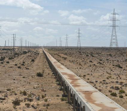
Source: The world’s longest conveyor belt system of 61 miles to convey phosphate ore to the sea (atlasobscura.com)
Preface. Phosphate is absolutely essential for both plants and animals. It’s estimated that Morocco has of 75-85% of phosphate reserves that might last for 300-400 years. Or peak in 25 years. Walan (2014) has estimates of researchers who’ve predicted peak phosphorus. But peak production will come early if Morocco and other key places experience supply chain failures, wars, economic depressions, lack of water, difficulty removing cadmium which is very toxic to plants.
China is the world’s largest producer of phosphate rock (48% of the world’s supply in 2013). It also uses a large amount of phosphorus to sustain its growing population. But China’s reserves of phosphorus, a key element for growing food, could be exhausted within the next 35 years if the country maintains its current production rate (Liu 2016).
Inevitably, the combination of rising cost and declining oil will force phosphate production to peak and then decline, even in Morocco (Bardi 2009).
If no action is taken decades before the anticipated peak, a hard-landing response to peak phosphorus is likely to result in a situation of (Cordell 2011c):
• increased energy and raw material consumption
• increased production, processing and transport costs
• increased generation of waste and pollution
• further short-term price spikes
• long-term trend of increased mineral phosphate prices
• increased geopolitical tensions
• reduced farmer access to fertilizer markets
• reduced global crop yields
• increased global hunger
Phosphorus may be the 11th most common element on earth, but each of these factors shrinks the amount available by further and further amounts until only a tiny amount is available for consumption:
1) Sufficient concentration of P
2) Found and physically accessible
3) Economically, energetically, legally, and geopolitically feasible
4) Available for fertilizer minus substantial mine-to-field losses
5) Plant available (P in soil solution)
6) Available for food minus substantial field-to-food losses
7) Available for consumption (minus food waste)
Clearly wars, supply chain failures, energy shortages / crisis, depressions, and more will also limit production.
2020. Researchers quantify worldwide loss of phosphorus due to soil erosion for the first time. More than 50% of global phosphorus loss in agriculture is due to soil erosion. Africa, Eastern Europe & South America have the greatest phosphorus losses—with limited options for solving the problem because fertilizers are too expensive for most farmers. Also, Africa has too little green fodder and too little animal husbandry to replace mineral fertilizers with manure and slurry.
It’s important to note that many of these assume production at current rates. But as human population continues to grow exponentially, the rate of extraction is likely to increase, not remain the same as the year of publication. The aim of this study is not to provide accurate predictions of future production of phosphate rock, and certainly not to foretell a date of a peak in production. What this study does attempt to show is that large global reserves of phosphate rock do not necessarily mean large annual production.
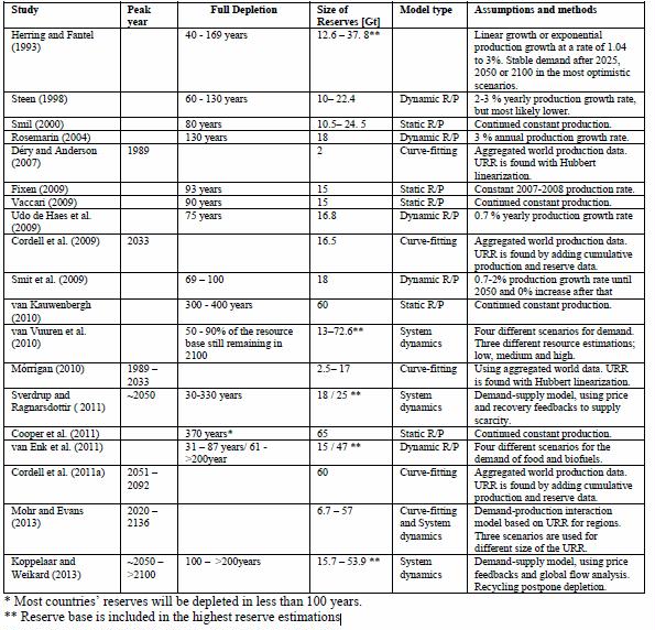
Table 1. Main features of previous studies on phosphate rock depletion and production. * Most countries’ reserves will be depleted in less than 100 years. ** Reserve base is included in the highest reserve estimations
We conclude that the total estimated recoverable amounts of phosphate rock will likely not be the most important limiting factor for the global production in the near future, but what is commonly neglected is that the global supply could come to rely almost completely on one single country, namely Morocco. This means that potential bottlenecks and concerns about phosphate rock production need to be analyzed in the context of the individual countries, in particular Morocco. A main question for further research is if it is possible and even desirable, both for Morocco and the importing countries, that production in Morocco should increase as much as are implicitly indicated in some projections for future phosphate rock production. Also, even if the whole Moroccan current reserves estimate is extractable, it is still a risk that global production will experience a peak as a result of the declining production in China.
Future demand, as well as the quantities of phosphate rock available for extraction is highly uncertain, but what is absolutely clear is that the current depletion of phosphate rock cannot go on forever and a more sustainable use of the essential element should be desired for a multitude of reasons. Although the future of phosphate rock production appears uncertain, even the possibility of reaching a “peak phosphorus” calls for a timely transition to a more sustainable use of the resources, with more widespread reuse, recycling and higher efficiency in use of fertilizers as potential mitigation measures to depletion.
For mineral resources, such as phosphate rock, high-grade mineral ores exist in finite quantities and extraction will eventually lead to an exhaustion of the resources that are economic to extract, at the same time as demand for minerals will likely continue to rise (May et al., 2012). Easy extractable deposits of phosphate rock, with a high content of P2O5, are often used first, while low P2O5 content deposits results in more impurities and higher production costs (Van Kauwenbergh 2010). Some studies claim that global concentrations have been, and are currently, declining steadily (Schröder et al., 2009; Cordell et al., 2009; Vaccari 2011). Such a trend imply that the “easy deposits have already been exhausted and that future production would be forced to develop lower quality deposits with more associated costs and challenges (UNEP, 2011). This has been described as a vital mechanism behind the generation of production peaks (Bardi, 2009).
Phosphorus (P) is among the most abundant elements and is ranked as the 11th most common in the earth’s crust (Krauss et al., 1984), and the 13th most common in seawater (Smil 2000). However, it does not occur in its elemental form in nature due to high reactivity. About 95% of all crustal phosphorus is estimated to be bound in different forms of phosphate apatite minerals of which there are more than 200 known variants (Krauss et al., 1984). Phosphate rock deposits that are interesting for mining usually only occur under special conditions in some specific areas as a result of the phosphorus cycle (Filippelli 2011; Krauss et al., 1984). The main phosphate rock deposits are either sedimentary or igneous, each with different mineralogical, structural, and chemical properties (Van Enk et al., 2011). Marine sedimentary deposits account for 80% of the global phosphate rock production, with large producers such as China, Morocco, U.S. and Tunisia. Sedimentary phosphate rock ores commonly have a P2O5 content of around 30-35% (Krauss et al., 1984). Igneous deposits are low grade in comparison, with a P2O5 content of often less than 5%, but can be upgraded through beneficiation to 35-40% or even higher. While igneous sources contribute with 15-20% of current production, they constitute much smaller fractions of estimated resources. In contrast to sedimentary phosphate rocks, igneous deposits are generally free from pollutants such as radionuclides and heavy metals (Smit et al., 2009). Igneous deposits can mainly be found in countries like Russia, Brazil, and South Africa.
Data availability of reserves and resources of phosphate rock is often poor, in part as mining companies and fertilizer industry have limited interest in making detailed data publicly available, thus forcing analysts to rely of 2nd and 3rd hand information (Cordell 2011; Gilbert 2009). It is also sometimes argued that the phosphate rock deposits in countries like Morocco are not fully explored, since mining companies refrain from expensive exploration of potential reserves that are not expected to be put in production in the near term (Van Kauwenbergh 2010). It also appears like reserve data from China excludes smaller mines, implying that actual reserves might be larger than officially reported (Cordell et al., 2009). Another potential source of misconceptions is that reserve data is sometimes presented as phosphate rock ore and sometimes phosphate rock concentrate. Reserves specified in tons of phosphate rock are often assumed to be the same as the recoverable amount of phosphate rock concentrate, even if reserves often actually are phosphate rock ore that must be beneficiated in order to be sold, which normally requires a P2O5 content of 30% (Edixhoven et al., 2013).
The global resources are estimated by the USGS to be about 300 Gt of phosphate ore, out of which about 67 Gt are considered currently economically recoverable reserves (Jasinski, 2013a). According to Edixhoven et al. (2013), the USGS reserve data is routinely assumed to be listed as phosphate rock concentrate, while it appears that USGS often list reserves in terms of ore. Edixhoven et al. (2013) also claims that more than half of the phosphate rock concentrate in the resources consists of the reserves.
USGS estimates have remained constant for many countries despite continuous production, while other countries have made significant changes in reserves. The USGS reserve estimates from 2001 to 2013 is depicted in Figure 1. The most notable change can be seen from 2010 to 2011 when the estimated reserves in Morocco was multiplied many times, leading to Morocco now comprising 75% of the global reserves. However, it appears questionable whether all this is truly recoverable at current prices (Edixhoven et al., 2013; GPRI 2010).
Others argue that much more phosphorus is extractable, pointing to potentially massive quantities available in sea beds, continental shelves or even the sea water itself. Marine phosphate mining has never been done in large scale and the impact intensive dredging could have on the marine environment is unclear (Filippelli 2011). Consequently, environmental impacts have to be carefully examined before oceanic mining can be undertaken (Scholz 2013). Similar to many other elements, seawater is sometimes argued to be a more or less infinite phosphorus resource (IFA, 1998). The same argument is commonly presented for lithium, which is discussed by Vikström et al. (2013), who give an example of extracting all the lithium in 300,000 km2 of seawater, corresponding to the average discharge of the river Nile, would give roughly 20,000 tons of lithium per year. Since the sea water contains less P than Li, the same flow of seawater would contain the equivalent of about 11,000 tons per year, which is less than 0.1% of the current global phosphorus production. Considering the phosphorus would also need to be extracted from these immense amounts of water, with unavoidable losses, production from seawater at significant levels near the current or projected future demand must be considered very unlikely, even if this type of production were to come to occur at large scale.
Global phosphorus production
Phosphate rock mining originally started in South Carolina 1867 for manufacturing of phosphate fertilizers (Van Kauwenbergh 2010). In the early 20th century, new complex fertilizers were created that contained phosphoric acid, as well as ammonium nitrate and potassium chloride, commonly called NPK fertilizers (UNEP/UNIDO 2000). In the 1960s, new high yielding crop varieties were introduced, which contributed to large increases in crop production (Evenson 2003). What is sometimes neglected is that these varieties only give high yields if they can extract more nutrients from the soil and these new varieties, together with increased use of irrigation, also led to an increased use of fertilizer (IFA 1998). Phosphate rock production grew quickly and appeared to reach a peak in production in 1988 as a result of decreasing demand and production after the fall of the Soviet Union that coincided with an increased awareness of issues with eutrophication (Cordell et al., 2009; IFA, 2011, 1998).
In recent years, production has again started to rise, for reasons such as a growing global population, a sharp increase in the consumption of meat and dairy products, especially in growing economies such as China and India, as well as an increased biomass production for bioenergy purposes (Cordell et al., 2009). A more extensive description of phosphorus usage through history can be found in Ashley et al. (2011) or Cordell et al. (2009).
Phosphate rock is currently mined in more than 30 countries worldwide, but very few countries make up most of the total production (EcoSanRes 2008). The U.S. has dominated production historically, but appears to have peaked in production in 1980 at a production of 54.6 Mt of phosphate rock concentrate, and has fallen to almost half of this level (Déry 2007). The former Soviet Union countries used to be large producers, but have now fallen to around 5% of global production.
China is currently the largest producer in the world, accounting for 89 Mt or 43% of the total production of phosphate rock concentrates in 2012. China accounts for most of the sharp increase in production that has taken place since 2000.
After China, the largest producers are the U.S. and Morocco with roughly 14% of the global output each (Jasinski 2013a). Other important producers are primarily found in the Middle East North Africa (MENA) region with countries like Tunisia, Jordan, Egypt, Israel, Syria, Saudi Arabia, and Algeria. The MENA region, including Morocco, currently contributes with about one quarter of the global production.
Since the phosphate price increased rapidly in 2007, several new deposits have been explored to boost production. One frontier region is Morocco, where in the national Moroccan Phosphates Company (OCP) stated in 2010 that they were to almost double production to 55 Mt/year by 2020, by opening four new mines (OCP 2010). However, the annual report from 2011 is not as ambitious and expects an increase of 20 Mt by 2020 (OCP 2011). Other recent mining developments are taking place worldwide. In Namibia and New Zealand, companies want to start marine mining of phosphate rock sediment. New mines are also planned to be developed in Finland (1.5 Mt/year), Kazakhstan (1.0 Mt/year) and Saudi Arabia (1.5 Mt/year) (De Ridder et al., 2012).
In 2011, only about 17% of the produced phosphate rock concentrate was exported directly, with the largest share being upgraded to phosphoric acid or phosphate fertilizers (IFA 2014). The total global trade of all forms of phosphate was only 22.5 Mt P2O5 in 2011 (OCP 2011), which means that around 63% of the phosphorus was consumed locally in the producing countries. Of the global phosphorus trade, 9.8 Mt P2O5(43%) was in the form of phosphate rock (IFA 2014). Especially China and the United States consume most of their production domestically, why Morocco accounts for the bulk of the world’s exports to the countries dependent on imports and provides 36.7% of the global export market (OCP 2011). Following their expansion plans, Moroccan export share are expected to increase substantially.
This study makes no attempts to project future demand of phosphate rock. Some of the results in the models presented reach phosphate rock production many times higher than current levels, and depending on the development of factors such as global population, diets, efficiency and recycling of phosphorous, the demand of virgin phosphate rock can look very different in the future.
There are many potential bottlenecks that could limit production flows and these should be addressed in the context of the individual countries where the production is supposed to happen. If countries such as Morocco are expected to increase their phosphate rock production with several times the current production, issues such as local environmental impacts, water availability, access to energy and geopolitical issues should be addressed on a regional level. Also, food producers could become more or less completely dependent on phosphate rock from Morocco due to its large and increasing share of the export market, which could lead to something resembling a monopolistic situation for Morocco in the future with associated risks (Elser and Bennett, 2011).
One important aspect is that the countries responsible for the phosphate rock mining will inevitably face local environmental impacts. Most phosphate rock is mined using large scale surface mining, which tend to have large impacts on the environment as it disturbs local landscape, and a wide range of other local environmental impacts can follow, such as water contamination, air emissions, noise and waste generation (UNEP, 2001).
Both phosphate rock production and beneficiation is highly water intensive, and water scarcity may essentially limit the beneficiation in dry areas (Van Kauwenbergh 2010). Many countries that produce phosphate rock, such as countries in the MENA region, already suffer from a shortage of fresh water (De Ridder 2012). In Morocco, most water is currently used for agriculture, out of which 30% is taken from the groundwater, often in an unsustainable way, and the groundwater table has fallen by an average of 1.5 meters per year since 1969 (UNEP, 2009). Energy intensive desalination plants are built by the national Moroccan phosphates company OCP to meet their need for water (OCP 2011).
Access to energy, especially oil, has been pointed out as a potential problem in the future as mining and fertilizer production rely on cheap oil and higher oil prices with associated supply chain effects caused by peak oil could increase production costs (Cordell 2009; Fantazzini 2011; Hanjra and Qureshi, 2010). For individual countries to be able to produce large amounts of phosphate rock, or products based on phosphorus, they will need large amounts of oil.
Geopolitical problems and civil unrest is a potential issue for phosphate rock production. The Arab spring, starting at the end of 2010, affected phosphate rock supply as production fell in several important producing countries in the MENA region, and the protracted conflict in Syria continues to influence supply of phosphate (de Ridder et al., 2012). Although not affected much by the Arab spring, Morocco has seen strikes and protests over employment and wealth equity concerns, but has not experienced any major disruptions in production (Wellstead 2012). Another issue is that Western Sahara, currently contributing with about 10% of Morocco’s phosphate rock production, has been occupied by Morocco since 1975, creating a ground for potential future instabilities (Edixhoven 2013).
Phosphate rock of different origin varies widely in composition and contains different quantities of impurities, such as cadmium (IFA 1998). It is have been suggested that the high cadmium content in many phosphate rock deposits in Morocco may provide an incentive for declining demand for Moroccan phosphate rock in the future (De Ridder 2012).
The future of phosphate rock
The current waste of phosphorus fertilizer causes a great deal of environmental problems, and it is questionable if it is a good idea to extract all the phosphate rock reserves if it would still end up in lakes, streams and the sea. As more and more phosphorus have been added to the ecosystem, many lakes and coasts have seen an increased algae growth (De Ridder 2012), which in some cases have led to serious eutrophication and dead zones due to lack of oxygen (Ashley 2011; Elser 2012). Carpenter (2011) even considers that the planetary boundaries for eutrophication of freshwater due to phosphorus have already been exceeded. It is possible to recycle phosphorus from human excreta, manure and different types of waste products (Cordell 2011b) and efficiency improvements in production and usage of phosphorus could offer a possibility to postpone a potential production peak (Cordell 2013).
Perhaps most importantly, the rather enormous phosphate rock reserves in Morocco is not a reason enough to stop attempting to find solutions towards a more sustainable food and energy system.
Estimates of future production of phosphate rock vary greatly depending on models used and assumptions made. Simple curve fitting modelling on aggregated global production data constrained by current USGS reserve estimates suggest that global phosphate rock production could reach a peak about 70 years from now, while other models or other reserve estimates used paints widely different pictures.
References
Ashley, K., Cordell, D., Mavinic, D., 2011. A brief history of phosphorus: From the philosopher’s stone to nutrient recovery and reuse. Chemosphere 84, 737–746.
Bardi, U., 2005. The mineral economy: a model for the shape of oil production curves. Energy Policy 33, 53–61.
Bardi, U., 2009. Peak oil: The four stages of a new idea. Energy 34, 323–326.
Bardi, U., Lavacchi, A., 2009. A Simple Interpretation of Hubbert’s Model of Resource Exploitation. Energies 2, 646–661.
BGS, 2013. World mineral statistics archive. British Geological Survey. Available at: http://www.bgs.ac.uk/mineralsuk/statistics/worldArchive.html
Buckingham, D.A., Jasinski, S.M., 2012. Historical Statistics for Mineral and Material Commodities in the United States; Phosphate rock statistics. http://minerals.usgs.gov/minerals/pubs/historical-statistics/ds140-phosp.pdf
Carpenter, S.R., Bennett, E.M., 2011. Reconsideration of the planetary boundary for phosphorus. Environ. Res. Lett. 6, 014009.
Cooper, J., Lombardi, R., Boardman, D., Carliell-Marquet, C., 2011. The future distribution and production of global phosphate rock reserves. Resources, Conservation and Recycling 57, 78–86.
Cordell, D., Drangert, J.-O., White, S., 2009. The story of phosphorus: Global food security and food for thought. Global Environmental Change 19, 292–305.
Cordell, D., White, S., Lindström, T., 2011a. Peak phosphorus: the crunch time for humanity? The Sustainability Review. Available from http://thesustainabilityreview.org/peak-phosphorus-thecrunch-time-for-humanity/
Cordell, D., Rosemarin, A., Schröder, J.J., Smit, A.L., 2011b. Towards global phosphorus security: A systems framework for phosphorus recovery and reuse options. Chemosphere 84, 747–758.
Cordell, D., White, S., 2011c. Peak Phosphorus: Clarifying the Key Issues of a Vigorous Debate about Long-Term Phosphorus Security. Sustainability 3, 2027–2049.
Cordell, D., White, S., 2013. Sustainable Phosphorus Measures: Strategies and Technologies for Achieving Phosphorus Security. Agronomy 3, 86–116.
De Ridder, M., De Jong, S., Polchar, J., Lingemann, S., 2012. Risks and Opportunities in the Global Phosphate Rock Market: Robust Strategies in Times of Uncertainty. The Hague Centre for Strategic Studies (HCSS). Report No 17 | 12 | 12. ISBN/EAN: 978-94-91040-69-6
Déry, P., Anderson, B., 2007. Peak phosphorus. Resilience. Available from:http://www.resilience.org/stories/2007-08-13/peak-phosphorus
EcoSanRes, 2008. Closing the Loop on Phosphorus. EcoSanRes Factsheet 4. Stockholm Environment Institute. Available at: http://www.ecosanres.org/pdf_files/ESR-factsheet-04.pdf
Edixhoven, J.D., Gupta, J., Savenije, H.H.G., 2013. Recent revisions of phosphate rock reserves and resources: reassuring or misleading? An in-depth literature review of global estimates of phosphate rock reserves and resources. Earth Syst. Dynam. Discuss. 4, 1005–1034.
Elser, J., Bennett, E., 2011. Phosphorus cycle: A broken biogeochemical cycle. Nature 478, 29–31.
Elser, J.J., 2012. Phosphorus: a limiting nutrient for humanity? Curr. Opin. Biotechnol. 23, 833–838.
Evenson, R.E., Gollin, D., 2003. Assessing the Impact of the Green Revolution, 1960 to 2000. Science 300, 758–762.
Fantazzini, D., Höök, M., Angelantoni, A., 2011. Global oil risks in the early 21st century. Energy Policy 39, 7865–7873.
Filippelli, G.M., 2011. Phosphate rock formation and marine phosphorus geochemistry: The deep time perspective. Chemosphere 84, 759–766.
Fixen, P.E., 2009. World Fertilizer Nutrient Reserves— A View to the Future. Better Crops, Vol. 93 No. 3 pp. 8-11.
Gilbert, N., 2009. Environment: The disappearing nutrient. Nature News 461, 716–718. Published in Resources Conservation and Recycling Volume 93, December 2014, Pages 178–187 http://dx.doi.org/10.1016/j.resconrec.2014.10.011
GPRI, 2010. GPRI Statement on Global Phosphorus Scarcity. http://phosphorusfutures.net/files/GPRI_Statement_responseIFDC_final.pdf
Hanjra, M.A., Qureshi, M.E., 2010. Global water crisis and future food security in an era of climate change. Food Policy 35, 365–377.
Herring, J.R., Fantel, R.J., 1993. Phosphate rock demand into the next century: Impact on world food supply. Nonrenewable Resour. 2, 226–246.
Hubbert, M.K., 1956. Nuclear energy and the fossil fuels. Report No. 95, Shell Development Company.
Hubbert, M.K., 1959. Techniques of prediction with application to the petroleum industry., Published in 44th Annual Meeting of the American Association of Petroleum Geologists. Shell Development Company, Dallas, TX.
Höök, M., Bardi, U., Feng, L., Pang, X., 2010. Development of oil formation theories and their importance for peak oil. Marine and Petroleum Geology 27, 1995–2004.
Höök, M., Li, J., Oba, N., Snowden, S., 2011. Descriptive and Predictive Growth Curves in Energy System Analysis. Natural Resources Research 20, 103–116.
IFA, 1998. The Fertilizer Industry, Food Supplies and the Environment. International Fertilizer Industry Association and United Nations Environment Programme, Paris, France.
IFA, 2011. Global Phosphate Rock Production Trends from 1961 to 2010. Reasons for the Temporary Set-Back in 1988-1994. International Fertilizer Industry Association (IFA). Paris, France.
IFA, 2014. Production and trade statistics. International Fertilizer Industry Association. http://www.fertilizer.org/ifa/HomePage/STATISTICS/Production-and-trade
Jakobsson, K., Bentley, R., Söderbergh, B., Aleklett, K., 2012. The end of cheap oil: Bottom-up economic and geologic modeling of aggregate oil production curves. Energy Policy 41, 860–870.
Jasinski, S.M., 2013a. Annual publication: Mineral Commodity Summaries: Phosphate Rock (1996-2013) U.S. Geological Survey. http://minerals.usgs.gov/minerals/pubs/commodity/phosphate_rock
Jasinski, S.M., 2013b. Minerals Yearbook, Phosphate Rock (1994-2013). U.S. Geological Survey. http://minerals.usgs.gov/minerals/pubs/commodity/phosphate_rock/
Koppelaar, R.H.E.M., Weikard, H.P., 2013. Assessing phosphate rock depletion and phosphorusrecycling options. Glob. Environ. Change, 23(6): 1454–1466.
Krauss, U.H., Saam, H.G., Schmidt, H.W., 1984. International Strategic Minerals Inventory SummaryReport – Phosphate, U.S. Geological Survey Circular 930-C. U.S. Department of the Interior.
May, D., Prior, T., Cordell, D., Giurco, D., 2012. Peak minerals: theoretical foundations and practicalapplication. Natural Resources Research, 21(1):43-60.
Mohr, S., Höök, M., Mudd, G., Evans, G., 2011. Projection of long-term paths for Australian coal production—Comparisons of four models. International Journal of Coal Geology 86, 329–341.
Mórrígan, T., 2010. Peak Phosphorus: A Potential Food Security Crisis. Global & International Studies, University of California. Santa Barbara, CA.
OCP, 2010. OCP Annual Report 2010. Office Chérifien des Phosphates.
OCP, 2011. OCP Annual Report 2011. Office Chérifien des Phosphates.
Pan, G., Harris, D.P., Heiner, T., 1992. Fundamental issues in quantitative estimation of mineral resources. Nat Resour Res 1, 281–292.
Rosemarin, A., 2004. The precarious geopolitics of phosphorous. Down to Earth. http://www.downtoearth.org.in/content/precarious-geopolitics-phosphorous
Rosemarin, A., De Bruijne, G., Caldwell, I., 2009. Peak phosphorus: the Next Inconvenient Truth. The Broker. http://www.thebrokeronline.eu/Articles/Peak-phosphorus
Scholz, R.W., Ulrich, A.E., Eilittä, M., Roy, A., 2013. Sustainable use of phosphorus: A finite resource. Science of The Total Environment 461–462, 799–803. Published in Resources Conservation and Recycling Volume 93, December 2014, Pages 178–187 http://dx.doi.org/10.1016/j.resconrec.2014.10.011
Scholz, R.W., Wellmer, F.-W., 2013. Approaching a dynamic view on the availability of mineral resources: What we may learn from the case of phosphorus? Global Environmental Change 23, 11–27.
Schröder, J.J., Cordell, D., Smit, A.L., Rosemarin, A., 2009. Sustainable Use of Phosphorus. Plant Research International, Wageningen UR and Stockholm Environment Institute (SEI), Report 357.
Smil, V., 2000. Phosphorus in the Environment: Natural Flows and Human Interferences. Annual Review of Energy and the Environment 25, 53–88.
Smit, A.L., Bindraban, P.S., Schröder, J.J., Conijn, J.G., Van der Meer, H.G., 2009. Phosphorus in the agriculture: global resources, trends and developments. Plant Research International, Wageningen UR. Report No. 282.
Steen, I., 1998. Phosphorus availability in the 21st century: Management of a non-renewable resource. Phosphorus & Potassium, Issue No:217. Available from: http://www.nhm.ac.uk/researchcuration/research/projects/phosphate-recovery/p&k217/steen.htm
Sverdrup, H.U., Ragnarsdottir, K.V., 2011. Challenging the planetary boundaries II: Assessing the sustainable global population and phosphate supply, using a systems dynamics assessment model. Appl. Geochem. 26, Supplement, S307–S310.
Udo de Haes, H.A., van der Weijden, W.J., Smit, A.L., 2009. Phosphate – from surplus to shortage. Steering Committee for Technology Assessment. Ministry of Agriculture, Nature and Food Quality, Utrecht.
UNEP, 2001. Environmental Aspects of Phosphate and Potash Mining. United Nations Environment Programme and International Fertilizer Industry Association, Paris, France.
UNEP, 2011. Phosphorus and Food Production, UNEP Year Book 2011.
UNEP/UNIDO, 2000. Mineral Fertilizer Production and the Environment. Part 1. The Fertilizer Industry’s Manufacturing Processes and Environmental Issues. United Nations Environment Programme Industry and the Environment United Nations Industrial Development Organization in collaboration with the International Fertilizer Industry, Paris, France.
USBM, 1993. Bureau of Mines Minerals Yearbook (1932-1993). http://minerals.usgs.gov/minerals/pubs/usbmmyb.html
USGS, 2013. Mineral Commodity Summaries 2013. Appendix C: Reserves and Resources. http://minerals.usgs.gov/minerals/pubs/mcs/2013/mcsapp2013.pdf
Vaccari, D.A., 2009. Phosphorus: A Looming Crisis. Sci. Am. 300, 54–59.
Vaccari, D.A., Strigul, N., 2011. Extrapolating phosphorus production to estimate resource reserves. Chemosphere 84, 792–797.
Van Enk, R.J., Van der Vee, G., Acera, L.K., Schuiling, R., Ehlert, P., 2011. The phosphate balance: current developments and future outlook. The ministry of Economic Affairs, Agriculture and nnovation initiated and finances InnovationNetwork. ISBN:978–90–5059–414–1
van Kauwenbergh, S., 2010. World Phosphate Rock Reserves and Resources.The International Fertilizer Development Center (IFDC).
van Vuuren, D.P., Bouwman, A.F., Beusen, A.H.W., 2010. Phosphorus demand for the 1970–2100 period: A scenario analysis of resource depletion. Glob. Environ. Change 20, 428–439.
Wellstead, J., 2012. Political Risks in MENA Phosphate Markets. Potash Invest. News. Available from: http://potashinvestingnews.com/4799-political-risks-mena-phosphate-markets-tunisiamorocco-jordan-syria-afric.html
Vikström, H., Davidsson, S., Höök, M., 2013. Lithium availability and future production outlooks.Applied Energy 110, 252–266.
Preface. I’m writing a book now which concludes that only biomass and biofuels can replace diesel and other fossil fuels. But 3 billion people are expected to arrive by 2050, consuming a good chunk of the biomass, plus it will be needed to replace half a million products made from fossil fuels, generate heat for homes and buildings, generate electricity, and dozens of other fossil fuel uses. Rural roads will take even more of a beating than they already are.
There are two articles below, the first about rural roads falling apart, and the second excerpts from a 302 page National Research Council study of Super Heavy commercial trucks that can weigh 2 million pounds. Ouch. Though after reading the whole damn thing, I never did found out the cost we taxpayers shoulder. But I did find what these super heavy objects were of interest, and show some of them below.
Picture this: County highway workers in bright safety vests pour scalding liquid rubber bandages on the road to cover the worst gashes. From above, it looks like skywriting — as if the bandages on the highway were spelling out a message for readers in the clouds.
The roads look like losers in a barroom brawl. Thick, jagged cracks run down the asphalt like scars, interrupted at points by bruised bumps. In some places, guardrails are tilted off their moorings like a pair of glasses knocked askew.
Rural roads are falling apart in small agricultural counties and towns across the Midwest and South, with eroding shoulders dangerous to the 80,000 pound trucks full of soybeans careening down the road. Reconstruction costs $300,000 per mile, and short-term patching $17,000 per mile.
Two-thirds of U.S. freight originates in rural areas where traffic volume has increased from heavy supersized tractor-trailers and farm equipment. In the spring thaw, melting will create soft spots easily damaged by heavy trucks.
These behemoths can produce 5,000 to 10,000 times the road damage of one car (TIC 2020). Although only 19% of American’s live in rural areas, they have 68% of total road miles.
Asphalt roads only have a lifespan of 30 years. Some county’s have roads far older than that.
The result is emergency closings and weight limits. Sometimes a farmer can’t easily move equipment from one field to another. Truckers have to make long detours to deliver feed and fertilizers. Trucks break down with broken axles, wrecked suspension systems, and flat tires.
States often don’t have the money to fix roads. For example, in Wisconsin the gas tax hasn’t gone up since 2006. Often there’s no state or federal assistance either.
NRC. 2015. Practices for Permitting Superheavy Load Movements on Highway Pavements. National Research Council, National Academies Press.
Maximum allowed superheavy vehicle weight. 1 kip = 1,000 pounds
This report documents the practices followed in issuing permits for overweight and superheavy commercial vehicles (SHCVs) or “superloads.” These are trucks that exceed the thresholds set for overweight vehicles allowed to operate with annual permits throughout state highway networks. This synthesis collected detail on the practices that U.S. states and Canadian provinces use. It focuses on SHCV issues related to pavements.
The GVW of the heaviest SHCV ever permitted by some agencies exceeds 2 million pounds
570,000 pound vehicle carrying an electrical anode used in the copper refining process. It was subjected to a bridge analysis, but not to a pavement analysis. It traveled from Nevada to Miami through Arizona
900,000 pound water purification vessel used in oil refining
A massive 900,000 pound water purification vessel used in oil refining was transported from its manufacturing origin in Portland through Oregon, Idaho, and Montana to its final destination in Alberta, Canada. The fee levied was just $4.26/mile for the entire vehicle. No seasonal restrictions were placed on the movement of this load because it was determined that the subgrade soil conditions encountered were relatively dry and therefore not susceptible to frost heave and/or spring thaw. The move took place in November 2013, during which frost and non-frost conditions were encountered. The vessel was delivered by Columbia River barge to Umatilla, Oregon, traveled for a short distance east on I-84, and then followed secondary roads south to the Idaho border near Ontario, Oregon. The vehicle had an overall length of 375 ft, 4 in. and a width of 22 ft, 2 in. Its GVW was 900 kips and its maximum tandem axle load was 44.75 kips. It was equipped with 32 axles and its maximum tire unit load was 604 lb/in. It was propelled by two pusher tractors and one pull tractor. No pavement analysis was conducted for its impact on the I-84 continuous reinforced concrete pavement.
1.2 million pound transformer moving on Texas roads
This 1.2 million pound truck is hauling a transformer from East Houston to Flat Rock, Texas, in August 2014. It had a total of 31 axle assemblies and measured 320 ft, 4 in. in length and 20 ft, 3 in. in width. The picture was taken on FM Road 3009 in Bexar County, Texas. Each trailer axle assembly consisted of two 4-tire axles side-by-side, taking the width of two adjacent roadway lanes. The heaviest axle assembly of this vehicle was 48,000 lb divided among eight tires. The move involved flag vehicles and police escorts. The permit fee charged for this vehicle was $935 and stipulated that the hauler is liable of any infrastructure damage.
The practices of permitting superheavy commercial vehicles (SHCVs) in the United States varies widely between agencies in terms of both the criteria used to define them, the analysis details for evaluating their impact on pavements, and the fees levied for permitting them.
The gross vehicle weight (GVW) thresholds used to define SHCVs vary from 120 kips to 254.3 kips. Axle load limits by configuration also vary, ranging from 20 to 29 kips for single axles on dual tires, from 34 to 60 kips for tandem axles on 8 tires, and from 50 to 81 kips for tridem axles on 12 tires. In addition, some agencies set limits on the tire weight per unit width (i.e., it varies between 500 and 800 lb/in.), whereas others do not. This obvious lack of uniformity in weight regulations reduces the weights of SHCVs traveling through multiple jurisdictions to the least common set of rules in effect through the jurisdictions involved and imposes a considerable administrative burden on shipping companies.
The literature review also suggests that SHCV single-trip fees vary considerably among the 62 jurisdictions in North America (i.e., 50 states, the District of Columbia, ten Canadian provinces, and the Yukon Territory): • Twenty-three (37%) levy SHCV permit fees that are a function of weight-distance, typically in the form of $/ton/ mile for GVW exceeding a certain value. Interestingly, some of the states that use weight-distance taxes do not use the same approach for levying SHCV permit fees. This fee ranges from $0.006/ton/mi to $0.2/ton/mi with an average value of about $0.049/ton/mi. • Fifteen (24%) levy SHCV permit fees that are related to GVW per axle weight alone and do not consider the distance traveled by the vehicles. • Eight (13%) levy a flat SHCV permit fee that ranges from $5 to $550, regardless of any pavement usage indicators, that is the weight of the vehicle or the distance traveled. • Seven (11%) levy a processing fee and may add an infrastructure usage fee after studying SHCVs on a case-bycase basis. • Two jurisdictions (3%) levy a flat fee and the cost of repairing the infrastructure from any damage rather than the cost infrastructure utilization from SHCV movement.
Thirty-eight agencies responded as to whether or not they conduct pavement analysis as part of their SHCV permit process. Of those, five (13%) always do (Delaware, Missouri, Louisiana, Tennessee, and Vermont), 15 (40%) do so depending on the circumstances (Arizona, Colorado, Iowa, Illinois, Indiana, North Carolina, North Dakota, Oregon, Washington State, Wisconsin, Wyoming, Texas, Virginia, British Columbia, and Ontario), whereas the remaining 18 agencies (47%) never perform such an analysis. The majority of the agencies that perform pavement analysis do so when dealing with a vehicle exceeding their definition of a SHCV. Details of pavement analysis performed were provided by 15 states. Their majority uses either their own in-house developed mechanistic empirical pavement analysis approach or the mechanistic methods developed by industry (i.e., Asphalt Pavement Association and Portland Cement Association). Several agencies indicated that they use the 1993 AASHTO Guide for the Design of Pavement Structures and characterize the truck loads in terms of equivalent single axle loads. None of the responding agencies uses the Mechanistic-Empirical Pavement Design Guide for analyzing the impact of SHCV. Additional details on the pavement analysis performed by the 15 responding states suggest that their majority uses representative thickness and layer/subgrade moduli, and consider the entire length of the SHCV. About half consider only one wheel path and the actual number of tires in the wheel path and the tire inflation pressure, while approximately 25% consider the actual vehicle speed. Furthermore, only four of the 15 responding agencies consider the stability of the pavement subgrade and of those one indicated using a Mohr– Coulomb type of analysis and another using a slope-stability numerical method type of analysis. The number of SHCV permits issued annually varies between agencies and to a large extent depends on their definition of SHCVs. The range is from fewer than 100 to more than 10,000 per year.
There have been regional efforts to establish uniform heavy truck permitting regulations in the United States, whereby a permit issued by one state is accepted for travel in other states. Twelve western states, under the auspices of the Western Association of State Highway and Transportation Officials (WASHTO), Arizona, Colorado, Idaho, Louisiana, Montana, New Mexico, Nevada, Oklahoma, Oregon, Texas, Utah, and Washington, agreed on a uniform set of truck weight regulations that allow trucks permitted in one of these states to legally operate throughout the rest. In summary, these limits consist of a GVW of 160 kips; tire weights of 600 lb/in. of width; overall consecutive axle weight limits governed by the Bridge Formula; and axle configuration weight limits of 21.5, 43, and 53 kips for single, tandem, and tridem axles, respectively.
The literature review suggests that SHCV single-trip fees vary widely between the 62 jurisdictions in North America (i.e., 50 states, the District of Columbia, ten Canadian provinces, and the Yukon Territory): • Twenty-three (37%) levy SHCV permit fees that are a function of weight-distance, typically in the form of $/ton/mile for GVW exceeding a certain value. Interestingly, some of the states that use weight-distance taxes do not use the same approach for levying SHCV permit fees. This fee ranges from $0.006/ton/mi to $0.2/ton/mi, with an average value of about 0.049/ton/mi. • Fifteen (24%) levy SHCV permit fees that are related to GVW/axle weight alone and do not consider at all the distance traveled by the vehicles. • Eight (13%) levy a flat SHCV permit fee that ranges from $5 to $550 regardless of any pavement usage indicators; that is, the weight of the vehicle or the distance traveled. • Seven (11%) levy a processing fee and may add an infrastructure usage fee after studying SHCVs on a case-by-case basis.
Two jurisdictions (3%) levy a flat fee and the cost of repairing the infrastructure from any damage rather than the cost infrastructure utilization from SHCV movement.
The definition of a SHCV or “superload” varies significantly among jurisdictions. Sixteen of the responding agencies (41%) define SHCV in terms of GVW alone, five (13%) use GVW and axle loads regardless of axle spacing, and another five (13%) use GVW and axle loads as a function of axle spacing. Interestingly, the remaining 13 responding agencies (33%) use an alternative definition involving vehicle size, tire loading, axle spacing, and roadway condition.
Thirty-eight agencies responded as to whether or not they conduct pavement analysis as part of their SHCV permit process. Of those, five (13%) always do (Delaware, Missouri, Louisiana, Tennessee, and Vermont), 15 (40%) do so depending on the circumstances (Arizona, Colorado, Iowa, Illinois, Indiana, North Carolina, North Dakota, Oregon, Washington, Wisconsin, Wyoming, Texas, Virginia, British Columbia, and Ontario), whereas the remaining 18 agencies (47%) never perform such an analysis. The majority of the agencies that perform pavement analysis do so when dealing with a vehicle exceeding their definition of a SHCV. Details on the pavement analysis performed were provided by 15 states. Their majority uses either their own in-house developed mechanistic-empirical pavement analysis approach or the mechanistic methods developed by industry. Several agencies indicated that they use the 1993 AASHTO Guide for the Design of Pavement Structures and characterize the traffic in terms of equivalent single axle loads. None of the responding agencies uses the Mechanistic-Empirical Pavement Design Guide for analyzing the impact of SHCVs.
Additional details on the pavement analysis performed by the 15 responding states suggest that the majority use representative thickness and layer/subgrade moduli and consider the entire length of the SHCV. About half of them consider only one wheel path, the actual number of tires in the wheel path, and the tire inflation pressure, while approximately 25% consider the vehicle speed. Furthermore, only four of the 15 responding agencies consider structural failure of the pavement layers and subgrade as part of the SHCV permitting analysis. Only two of these four states gave details on the actual method used for analyzing the structural stability of the pavement layers.
The results of the survey questionnaire confirmed the findings of the literature review on the various methodologies agencies use for computing SHCV permit fees. Fifteen of the 46 responding agencies (33%) use a GVW-distance-traveled approach (Alabama, Florida, Illinois, Ohio, Missouri, Montana, North Dakota Tennessee, Utah, Vermont, Washington, West Virginia, Wyoming, British Columbia, and Ontario), two use a pavement damage-distancetraveled approach (Arizona and Oregon), another two use a number of axles-distance-traveled approach (Idaho and New Jersey), while 19 (41%) use a different methodology.
The findings of this study suggest that the practice of permitting SHCVs could be significantly improved through further study of their impact on pavements and implementation of the results in establishing equitable permit fees that cover pavement utilization and/or damage.
INTRODUCTION
There is an increasing demand for highway transport of very large non-divisible shipments that not only exceed legal gross vehicle weight (GVW) and axle weight limits, but also exceed the special provisions that allow overweight vehicles to operate with routine annual permits. Such vehicles are typically allowed to operate under single-trip permits following an engineering analysis of their impact on the pavement infrastructure (pavements and bridges) on a specific route.
State and provincial practices on permitting such vehicles, henceforth to be referred to as superheavy commercial vehicles (SHCVs) or “superloads,” have a significant impact on both transportation efficiency and infrastructure condition.
The condition of the pavement infrastructure is affected where the fees collected for SHCV permitting do not cover the pavement damage cost caused by these vehicles.
The differences in weight limits between jurisdictions, even those that have common borders, are substantial. For example, a vehicle with a GVW between 150 and 199 kips crossing the Florida–Georgia border would require a SHCV permit review in Georgia but not in Florida, and would be required to have a unit tire weight of less than 550 lb/in. only in Florida, since Georgia does not have this requirement.
Similarly, a vehicle with a GVW between 144 and 191 kips crossing the Minnesota–Wisconsin border would require a SHCV permit review in Minnesota but not in Wisconsin, and would face different maximum permitted axle weights (e.g., tandem axle weights of 40 versus 60 kips and tridem axle weights of 60 versus 81 kips, respectively).
Clearly, there is a lack of uniformity in weight regulations for SHCVs between jurisdictions.
As mentioned earlier, the U.S. Congress recently authorized a Comprehensive Truck Size and Weight Limits Study (1) under MAP-21 funding (Moving Ahead for Progress in the 21st Century Act; Section 32801), with the following objectives: • Address the differences in safety risks, infrastructure impacts, and the effect on levels of enforcement between trucks operating at or within federal truck size and weight limits and trucks legally operating in excess of federal limits; • Compare and contrast the potential safety and infrastructure impacts of alternative configurations (including configurations that exceed current federal limits) to the current federal truck size and weight law and regulations; and • Estimate the effects of freight diversion resulting from these alternative configurations.
DEFINITION OF SUPERHEAVY COMMERCIAL VEHICLES
This section summarizes the survey results related to background questions and the way SHCVs are defined and permitted in each jurisdiction. 16 of the responding agencies (41%) define SHCV in terms of a maximum GVW alone. They vary widely from 120 to 500 kips, with the most frequent value being 200 kips. Five of the responding agencies (13%) reported that they define SHCV in terms of GVW and axle group limits regardless of axle spacing. The wide range of GVW and load limits is again evident; GVW limits range from 80 kips to 350 kips and tandem axle loads, for example, range from 34 kips to more than 60 kips. Another five of the responding agencies (13%) define SHCV in terms of GVW and axle group limits as a function of axle spacing. The distribution of these GVW limits, the axle group load limits, and the corresponding minimum axle spacings. In this case, GVWs vary from 100 to 254 kips, tandem load limits from 40 to 50 kips, whereas minimum tandem axle spacings vary from 6 to 12 feet.
The potato battery is a type of electrochemical battery, or cell. Certain metals (zinc in the demonstration below) experience a chemical reaction with the acids inside of the potato. This chemical reaction creates the electrical energy that can power a small device like an LED light or clock (SFF 2018).
The satirical Onion proposes powering cities on Potato Power. But why not — potatoes are renewable, unlike wind, solar, wave, nuclear, and all other contraptions that depend on fossils for every step of their life cycle.
KNOXVILLE, TN—In what many experts are hailing as a game changer in the field of renewable energy, scientists from the University of Tennessee unveiled Friday a 10-story-tall, 800,000-ton potato capable of powering an entire city. “Our tests have demonstrated this single potato can generate more than 3.5 gigawatts of clean, renewable electricity,” said civil engineering professor Lauren Donaldson, explaining that the colossal tuber, when connected to the electrical grid via one zinc and one copper electrode, could provide enough output to illuminate approximately 70 million standard light bulbs for more than a decade. “In theory, the nation’s energy infrastructure could be revolutionized simply by placing one of these gigantic potatoes next to every city in America. We believe it is entirely conceivable that within 20 years, this technology—perhaps supplemented by several similar-sized lemons connected via lengths of wire and paper clips—could be our primary source of electricity. One day, everything from home appliances to cars to factories may be potato-powered.” Donaldson added that her team’s potato also had the benefit of being largely pollution-free, as nearly 98 percent of its waste products would be fried-up and eaten afterward (The Onion 2020).
A new report from the Department of Energy has uncovered an unforeseen source of mechanical kinetic energy: our Founding Fathers spinning in their graves. “For decades, our nation has lamented the fact that John Adams is likely oscillating in his coffin,” said a spokesperson. “But we’re only now discovering that our Founding Fathers’ rotational exasperation at the state of America today is a source of clean, white-hot fuel, comparable to over 15,000 nuclear reactors. Environmental scientists were quick to remind reporters that from a Constitutional standpoint, of course we should respect the laws on which America was founded. But from a sustainability standpoint, they urged the public to do everything possible to anger the ghost of Benjamin Franklin. “This source of combustion was first ignited during the freeing of slaves, and boosted by women’s suffrage. But if we’re serious about fighting climate change, we recommend kicking the spinning up a notch by permanently banning all firearms, censoring large amounts of speech, and implementing fully-automated luxury space gay communism.”
In tubes and tanks under the chassis, something very like soapy water mixed
with hydrogen called sodium borohydride and similar to borax found in laundry
detergent, is being tested (Steen 2002). Of course, there are many
problems why this hasn’t worked out and probably never will.
Thermal depolymerization and landfills turn garbage into biogass. But
as energy declines, there will be less and less garbage, not only because there
won’t be the fuel to take it to a landfill, but people will be burning anything
they can get their hands on to cook and heat with.
Raindrop power
Researchers reported that a single drop can muster 140V, or enough power to
briefly light up 100 small LED bulbs. It’s far from being able to produce
continuous power. This system works with drops of the same size falling from
the same height and may not do as well otherwise, and degradation of surface
charge may reduce the generator’s efficiency with time. Meanwhile maybe someone
can build a miniature Las Vegas for mice (Delbert 2020).
Elon Musk’s hyperloop
Not going to happen for too many reasons to list. Just one is that because temperature ranges from 32 to 120 F, there’d need to be 6,000 expansion joints. If even one failed, disaster. The vacuum would be released. This 28 minute video explains this and much more at: https://www.youtube.com/watch?v=RNFesa01llk
It’s time to look at what we can gain from muscle power, which will have to
increasingly replace fossil fuels as they decline. This has the added bonus of helping to cope
with the obesity crisis. The authors estimate that an average American has 5
pounds of excess fat, which translates to 133,000 GJ of stored energy. Using
human muscle as an energy source has the added benefit of reducing heart
disease, strokes, and diabetes.
Gym members comprise a large potential muscle power workforce. Over 54
million people are members of a fitness center in the U.S. where their
potential electricity generating exercise is wasted. Instead, members do the opposite
and consume electricity, since equipment such as treadmills, ellipticals,
stationary bikes, and rowers are electric. And air conditioning to keep members
cool uses additional electricity.
This study looked at how much electric power could be generated by 40
members at a gym in South Carolina.
At best, 3-5% of the gym’s average daily electricity demand could be provided at a large cost. To convert the rowing machines to generate electricity would take 33 years to pay back, perhaps longer than a rowing machine will last
References
Carbajales-Dale, M., et al. 2018. Human powered electricity generation as a
renewable resource. BioPhysical Economics and Resource Quality.
Delbert, C. 2020. The Cool Way Scientists Turned Falling
Raindrops Into Electricity. Popular Mechanics.
Steen, M. 16 Sep 2002. A squeaky clean future for the car?
Reuters News Service.
Posted inFar Out|Taggedhyperloop, raindrop, soap|Comments Off on Far out power #2: Soap, Raindrops, Hyperloops, and Fitness Centers
Preface. Before sewage treatment, cities were hell-holes of foul smells from rotting human waste, industrial effluent, and garbage. Few people lived beyond 50 because of the many waterborne diseases. In fact, sewage and water treatment systems are the main reason lifespans nearly doubled (Garrett 2001). Here are just a few of the diseases possible from drinking untreated water: Adenovirus infection, Amebiasis, Campylobacteriosis, Cryptosporidiosis, Cholera, E. Coli 0157:H7, Giardiasis, Hepatitis A, Legioellosis, Salmonellosis, Vibrio infection, Viral gastroenteritis, free living amoebae (ADHS). For the full list of waterborne diseases, see post Water-borne diseases will increase as energy declines.
Nearly all sewage infrastructure is past its life-time, a good way to spend the remaining cheap oil before it becomes scarce.
Sewage is also a way to return nutrients back to the soil, especially finite phosphorus, which is eaten and excreted, treated, and lost to oceans and other waterways.
Today moving sludge from city sewage treatment farms works because of cheap energy. In the future energy crisis, that won’t be possible.
There are two articles below, one about sewage sludge for crops, and the other about sewage corrosion.
Human waste is a nutrient-rich substance that farmers around the world have spread on cropland for centuries. Every day, about 20 million gallons of sewage flows into the city of Tacoma’s wastewater treatment plants. The water is separated, treated, and discharged into the Puget Sound, which leaves behind sludge — a mix of human excrement, industrial waste, and everything else that ends up in sewers. The plants further treat the product to reduce pathogens, bacteria, heavy metals, and odors, and convert it into a fertilizer called biosolids, which is high in phosphorus, nitrogen, and other nutrients that help plants grow.
Over 50 percent of the approximately 130 million wet tons of sludge produced nationally each year is treated and applied to less than 1% of cropland. As a fertilizer, it’s popular because most wastewater treatment plants give it away for free or at prices less than the cost of synthetic fertilizers.
The Sierra club notes that it can contain up to 90,000 man-made chemicals and we don’t know what new chemicals are made synergistically by combining them. It’s not certain that biosolids are safe.
One of the most controversial piece of the sewage puzzle is the fact that factories, slaughterhouses, and other industrial facilities are allowed to discharge their waste into the taxpayer-funded sewer system.
Before the 1972 Clean Water Act, the waste industry largely burned it, but that often violates the Clean Air Act, Lewis said. Municipalities also tried dumping it in the ocean, but that created large dead zones. Then, in 1993, the EPA approved a proposal to spread it on land after it was treated. Sludge that isn’t turned into biosolids is landfilled or incinerated — both of which are expensive compared to spreading it on farmland.
The EPA only requires nine pollutants — all heavy metals — to be removed from biosolids, as well as living pathogens such as E. coli and Salmonella. Sludge may be treated by air drying, pasteurization, or composting. Lime is often used to raise the pH level to eliminate odors, and about 95 percent of pathogens, viruses, and other organisms are killed in the process, according to waste management industry officials.
Sewer systems are among the most critical infrastructure assets for modern urban societies and provide essential human health protection. Sulfide-induced concrete sewer corrosion costs billions of dollars annually and has been identified as a main cause of global sewer deterioration. Aluminum sulfate addition during drinking water production contributes substantially to the sulfate load in sewage and indirectly serves as the primary source of sulfide. This unintended consequence of urban water management structures could be avoided by switching to sulfate-free coagulants, with no or only marginal additional expenses compared with the large potential savings in sewer corrosion costs.
Sewer systems are corroding at an alarming rate, costing governments billions of dollars to replace. Differences among water treatment systems make it difficult to track down the source of corrosive sulfide responsible for this damage.
Urban sewer networks collect and transport domestic and industrial waste waters through underground pipelines to wastewater treatment plants for pollutant removal before environmental discharge. They protect our urban society against sewage-borne diseases, unhygienic conditions, and noxious odors and so allow us to live in ever larger and more densely populated cities. Today’s underground sewer infrastructure is the result of an enormous investment over the last 100+ years with, for example, an estimated asset value of one trillion dollars in the USA (Brongers). This equates to ~7% of its current gross domestic product. However, these assets are under serious threat with an estimated annual asset loss of around $14 billion in the United States alone. Sulfide-induced concrete corrosion is recognized as a main cause of sewer deterioration in most cases.
Many water utilities will need to upgrade both their water supply and wastewater service infrastructure over the next 10 to 15 years, which will require enormous capital investments.
References
ADHS. Waterborne diseases. Arizona Department of Health Services.
Brongers, M. P. H., et al. 2002. “Drinking water and sewer systems in corrosion costs and preventative strategies in the United States”. Federal Highway Administration Publication FHWA-RD-01-156, U.S. Department of Transportation, Washington, DC.
Preface. There are three articles below on this topic. Plus these articles in the news:
Nakagawa T et al (2021) The spatio-temporal structure of the Lateglacial to early Holocene transition reconstructed from the pollen record of Lake Suigetsu and its precise correlation with other key global archives: Implications for palaeoclimatology and archaeology. Global and Planetary Change
The team’s data show that the transition from the ice age to the post-glacial age was characterized by alternations between stable and unstable periods. The domestication of plants didn’t start when the warm climate was established in ca. 13,000 BC, but had to wait until the climate stopped oscillating in short intervals and large amplitudes in ca. 12,000 BC. Agriculture is a subsistence practice that requires planning. But to plan in advance, a stable future is important. When the climate was unstable, agriculture was too risky a practice because accurately predicting the weather in the future wasn’t possible, thus making it difficult to select appropriate crops for agriculture. In such climatic conditions, hunting-and-gathering was a more reasonable subsistence strategy than agriculture because the natural ecosystem consists of diverse species from which humans could expect “something” edible, as opposed to the farmlands. These new findings challenge the traditional view that agriculture was a revolutionary step forward for the history of humanity. Instead, agriculture and hunting-and-gathering were equally reasonable adaptation strategies, depending on whether the climate was stable or unstable. https://www.sciencedaily.com/releases/2021/07/210729095215.htm
2022 Dwindling Mississippi Grounds Barges, Threatens Shipments. Bloomberg. A logjam of more than 100 ships, tugboats and their convoys of barges in the shrinking Mississippi River is threatening to grind trade of grains, fertilizer, metals and petroleum to a halt. Drought has reduced water levels along the biggest US waterway by so much that vessels are running aground. The largest US barge operator, Ingram Barge Co, declared force majeure due to “near-historic” low water conditions on the Mississippi, the top route to get US grains and soybeans to the world market. Some 60% of all grain exported from the US is shipped on the Mississippi River. The logjam is coming at the worst time as the soybean and corn harvests are each about one-fifth complete and supplies will start piling up, and the river is also vital to transport fertilizer.
Earth’s dryland ecosystem covers 45% of the world’s surface and is home to around a third of its population who depend on these areas for their food and water.
This study found that as aridity increases, dryland ecosystems undergo a series of abrupt changes. This results first in drastic reductions in the capacity of plants to fix carbon from the atmosphere, then substantial declines of soil fertility, drought-tolerant plants replace food crops, and finally vegetation disappears under the most arid and extreme conditions and turns into a desert.
As aridification grows worse, the land becomes more vulnerable to erosion, soil biota maintaining the ecosystem decline, pathogens increase, crops fail.
More than 20% of land may cross these thresholds by 2100 due to climate change.
Climate disruptions to agricultural production have increased in the past 40 years and are projected to increase over the next 25 years. By 2050 and beyond, these impacts will be increasingly negative on most crops and livestock.
Many agricultural regions will experience declines in crop and livestock production from increased stress due to weeds, diseases, insect pests, and other climate change induced stresses.
Current loss and degradation of critical agricultural soil and water assets due to increasing extremes in precipitation will continue to challenge both rain-fed and irrigated agriculture
The rising incidence of weather extremes will have increasingly negative impacts on crop and livestock productivity because critical thresholds are already being exceeded.
Agriculture has been able to adapt to recent changes in climate; however, increased innovation will be needed to ensure the rate of adaptation of agriculture and the associated socioeconomic system can keep pace with climate change over the next 25 years.
Climate change effects on agriculture will have consequences for food security, both in the U.S. and globally, through changes in crop yields and food prices and effects on food processing, storage, transportation, and retailing. Adaptation measures can help delay and reduce some of these impacts.
The United States produces nearly $330 billion per year in agricultural commodities, with livestock accounting for half of that value. Production of all commodities will be vulnerable to direct impacts (from changes in crop and livestock development and yield due to changing climate conditions and extreme weather events) and indirect impacts (through increasing pressures from pests and pathogens that will benefit from a changing climate). Crop production projections often fail to consider the indirect impacts from weeds, insects, and diseases that accompany changes in both average trends and extreme events, which can increase losses significantly.
Rising average temperatures will increase crop water demand, increasing the rate of water use by the crop. Higher temperatures are projected to increase both evaporative losses from land and water surfaces and transpiration losses (through plant leaves) from non-crop land cover, potentially reducing annual runoff and streamflow for a given amount of precipitation.
By mid-century, when temperature increases are projected to be between 1.8°F and 5.4°F and precipitation extremes are further intensified, yields of major U.S. crops and farm profits are expected to decline. There have already been detectable impacts on production due to increasing temperatures.
One critical period in which temperatures are a major factor is the pollination stage; pollen release is related to development of fruit, grain, or fiber. Exposure to high temperatures during this period can greatly reduce crop yields and increase the risk of total crop failure. Plants exposed to high nighttime temperatures during the grain, fiber, or fruit production period experience lower productivity and reduced quality. These effects have already begun to occur; high nighttime temperatures affected corn yields in 2010 and 2012 across the Corn Belt. With the number of nights with hot temperatures projected to increase as much as 30%, yield reductions will become more prevalent.
Plants have specific temperature tolerances, and can only be grown in areas where their temperature thresholds are not exceeded. As temperatures increase over this century, crop production areas may shift to follow the temperature range for optimal growth and yield of grain or fruit. Temperature effects on crop production are only one component; production over years in a given location is more affected by available soil water during the growing season than by temperature, and increased variation in seasonal precipitation, coupled with shifting patterns of precipitation within the season, will create more variation in soil water availability.
Increasing temperatures cause cultivated plants to grow and mature more quickly. Crops, such as cereals, would grow more quickly, meaning less time for the grain itself to mature, reducing productivity. But because the soil may not be able to supply nutrients at required rates for faster growing plants, plants may be smaller, reducing grain, forage, fruit, or fiber production.
In vegetables, exposure to temperatures in the range of 1.8°F to 7.2°F above optimal moderately reduces yield, and exposure to temperatures more than 9°F to 12.6°F above optimal often leads to severe if not total production losses.
Temperature and precipitation changes will include an increase in both the number of consecutive dry days (days with less than 0.01 inches of precipitation) and the number of hot nights. The western and southern parts of the nation show the greatest projected increases in consecutive dry days, while the number of hot nights is projected to increase throughout the U.S. These increases in consecutive dry days and hot nights will have negative impacts on crop and animal production. High nighttime temperatures during the grain-filling period (the period between the fertilization of the ovule and the production of a mature seed in a plant) increase the rate of grain-filling and decrease the length of the grain-filling period, resulting in reduced grain yields. Exposure to multiple hot nights increases the degree of stress imposed on animals resulting in reduced rates of meat, milk, and egg production.
Climate change poses a major challenge to U.S. agriculture because of the critical dependence of the agricultural system on climate and because of the complex role agriculture plays in rural and national social and economic systems (Figure 6.2). Climate change has the potential to both positively and negatively affect the location, timing, and productivity of crop, livestock, and fishery systems at local, national, and global scales. It will also alter the stability of food supplies and create new food security challenges for the United States
Over time, climate change is expected to increase the annual variation in crop and livestock production because of its effects on weather patterns and because of increases in some types of extreme weather events.
Each crop species has a temperature range for growth, along with an optimum temperature.9 Plants have specific temperature tolerances, and can only be grown in areas where their temperature thresholds are not exceeded. As temperatures increase over this century, crop production areas may shift to follow the temperature range for optimal growth and yield of grain or fruit. Temperature effects on crop production are only one component; production over years in a given location is more affected by available soil water during the growing season than by temperature, and increased variation in seasonal precipitation, coupled with shifting patterns of precipitation within the season, will create more variation in soil water availability. The use of a model to evaluate the effect of changing temperatures
Key Message: Extreme Precipitation and Soil Erosion
Current loss and degradation of critical agricultural soil and water assets due to increasing extremes in precipitation will continue to challenge both rainfed and irrigated agriculture unless innovative conservation methods are implemented. Wind erosion could also increase in areas with persistent drought because of the reduction in vegetative cover.
Several processes act to degrade soils, including erosion, compaction, acidification, salinization, toxification, and net loss of organic matter. Several of these processes, particularly erosion, will be directly affected by climate change. Rainfall’s erosive power is expected to increase as a result of increases in rainfall amount in northern portions of the United States, accompanied by further increases in precipitation intensity. Projected increases in rainfall intensity that include more extreme events will increase soil erosion in the absence of conservation practices. Precipitation and temperature affect the potential amount of water available, but the actual amount of available water also depends on soil type, soil water holding capacity, and the rate at which water filters through the soil.
Iowa is the nation’s top corn and soybean producing state. These crops are planted in the spring. Heavy rain can delay planting and create problems in obtaining a good stand of plants, both of which can reduce crop productivity. In Iowa soils with even modest slopes, rainfall of more than 1.25 inches in a single day leads to runoff that causes soil erosion and loss of nutrients and, under some circumstances, can lead to flooding. Figure 6.9 shows the number of days per year during which more than 1.25 inches of rain fell is increasing.
A few of the ecosystem services provided by soils include:
the provision of food
wood
fiber (i.e. cotton)
raw materials
flood mitigation
recycling of wastes
biological control of pest
regulation of carbon and other heat-trapping gases
physical support for roads and buildings
cultural and aesthetic values
Productive soils are characterized by levels of nutrients necessary for the production of healthy plants, moderately high levels of organic matter, a soil structure with good binding of the primary soil particles, moderate pH levels, thickness sufficient to store adequate water for plants, a healthy microbial community, and the absence of elements or compounds in concentrations that are toxic for plant, animal, and microbial life.
Erosion is managed through maintenance of cover on the soil surface to reduce the effect of rainfall intensity. Studies have shown that a reduction in projected crop biomass (and hence the amount of crop residue that remains on the surface over the winter) will increase soil loss.
Key Message: Weeds, Diseases, and Pests
Many agricultural regions will experience declines in crop and livestock production from increased stress due to weeds, diseases, insect pests, and other climate change induced stresses.
The growth of atmospheric CO2 concentrations has a disproportionately positive impact on several weed species. This effect will contribute to increased risk of crop loss due to weed pressure.
Weeds, insects, and diseases already have large negative impacts on agricultural production, and climate change has the potential to increase these impacts. Current estimates of losses in global crop production show that weeds cause the largest losses (34%), followed by insects (18%), and diseases (16%). Further increases in temperature and changes in precipitation patterns will induce new conditions that will affect insect populations, incidence of pathogens, and the geographic distribution of insects and diseases. Increasing CO2 boosts weed growth, adding to the potential for increased competition between crops and weeds. Several weed species benefit more than crops from higher temperatures and CO2 levels.
One concern involves the northward spread of invasive weeds like privet and kudzu, which are already present in the southern states. Changing climate and changing trade patterns are likely to increase both the risks posed by, and the sources of, invasive species. Controlling weeds costs the U.S. more than $11 billion a year, with most of that spent on herbicides. Both herbicide use and costs are expected to increase as temperatures and CO2 levels rise. Also, the most widely used herbicide in the United States, glyphosate, loses its efficacy on weeds grown at CO2 levels projected to occur in the coming decades. Higher concentrations of the chemical and more frequent sprayings thus will be needed, increasing economic and environmental costs associated with chemical use.
Insects are directly affected by temperature and synchronize their development and reproduction with warm periods and are dormant during cold periods. Higher winter temperatures increase insect populations due to overwinter survival and, coupled with higher summer temperatures, increase reproductive rates and allow for multiple generations each year. An example of this has been observed in the European corn borer (Ostrinia nubialis) which produces one generation in the northern Corn Belt and two or more generations in the southern Corn Belt. Changes in the number of reproductive generations coupled with the shift in ranges of insects will alter insect pressure in a given region.
Key Message: Heat and Drought Damage
The rising incidence of weather extremes will have increasingly negative impacts on crop and livestock productivity because critical thresholds are already being exceeded.
Climate change projections suggest an increase in extreme heat, severe drought, and heavy precipitation. Extreme climate conditions, such as dry spells, sustained droughts, and heat waves all have large effects on crops and livestock. The timing of extreme events will be critical because they may occur at sensitive stages in the life cycles of agricultural crops or reproductive stages for animals, diseases, and insects. Extreme events at vulnerable times could result in major impacts on growth or productivity, such as hot-temperature extreme weather events on corn during pollination. By the end of this century, the occurrence of very hot nights and the duration of periods lacking agriculturally significant rainfall are projected to increase. Recent studies suggest that increased average temperatures and drier conditions will amplify future drought severity and temperature extremes. Crops and livestock will be at increased risk of exposure to extreme heat events. Projected increases in the occurrence of extreme heat events will expose production systems to conditions exceeding maximum thresholds for given species more frequently.
California’s Wine, Fruit, & Nut production will begin declining as soon as 2050
In fact, it’s already happening. In 2000, the number of chilling hours in some regions was 30% lower than in 1950. A warmer climate will affect growing conditions, and the lack of cold temperatures may threaten perennial crop production (Figure 6.6), which have a winter chilling requirement (expressed as hours when temperatures are between 32°F and 50°F) ranging from 200 to 2,000 cumulative hours. Yields decline if the chilling requirement is not completely satisfied, because flower emergence and viability is low. Projections show that chilling requirements for fruit and nut trees in California will not be met by the middle to the end of this century.
Impacts on Animal Production
Animal agriculture is a major component of the U.S. agriculture system. Changing climatic conditions affect animal agriculture in four primary ways: 1) feed-grain production, availability, and price; 2) pastures and forage crop production and quality; 3) animal health, growth, and reproduction; and 4) disease and pest distributions. The optimal environmental conditions for livestock production include temperatures and other conditions for which animals do not need to significantly alter behavior or physiological functions to maintain relatively constant core body temperature.
Optimum animal core body temperature is often maintained within a 4°F to 5°F range, while deviations from this range can cause animals to become stressed. This can disrupt performance, production, and fertility, limiting the animals’ ability to produce meat, milk, or eggs. In many species, deviations in core body temperature in excess of 4°F to 5°F cause significant reductions in productive performance, while deviations of 9°F to 12.6°F often result in death. For cattle that breed during spring and summer, exposure to high temperatures reduces conception rates. Livestock and dairy production are more affected by the number of days of extreme heat than by increases in average temperature. Elevated humidity exacerbates the impact of high temperatures on animal health and performance.
Animals respond to extreme temperature events (hot or cold) by altering their metabolic rates and behavior. Increases in extreme temperature events may become more likely for animals, placing them under conditions where their efficiency in meat, milk, or egg production is affected. Projected increases in extreme heat events will further increase the stress on animals, leading to the potential for greater impacts on production. Meat animals are managed for a high rate of weight gain (high metabolic rate), which increases their potential risk when exposed to high temperature conditions. Exposure to heat stress disrupts metabolic functions in animals and alters their internal temperature when exposure occurs. Exposure to high temperature events can be costly to producers, as was the case in 2011, when heat-related production losses exceeded $1 billion.
Livestock production faces additional climate change related impacts that can affect disease prevalence and range. Regional warming and changes in rainfall distribution have the potential to change the distributions of diseases that are sensitive to temperature and moisture, such as anthrax, blackleg, and hemorrhagic septicemia, and lead to increased incidence of ketosis, mastitis, and lameness in dairy cows.
Goats, sheep, beef cattle, and dairy cattle are the livestock species most widely managed in extensive outdoor facilities. Within physiological limits, animals can adapt to and cope with gradual thermal changes, though shifts in thermoregulation may result in a loss of productivity. Lack of prior conditioning to rapidly changing or adverse weather events, however, often results in catastrophic deaths in domestic livestock and losses of productivity in surviving animals.
Key Message: Rate of Adaptation
Agriculture has been able to adapt to recent changes in climate; however, increased innovation will be needed to ensure the rate of adaptation of agriculture and the associated socioeconomic system can keep pace with climate change over the next 25 years.
In the longer term existing adaptive technologies will likely not be sufficient to buffer the impacts of climate change without significant impacts to domestic producers, consumers, or both. Limits to public investment and constraints on private investment could slow the speed of adaptation. Adaptation may also be limited by the availability of inputs (such as land or water), changing prices of other inputs with climate change (such as energy and fertilizer), and by the environmental implications of intensifying or expanding agricultural production.
In addition to regional constraints on the availability of critical basic resources such as land and water, there are potential constraints related to farm financing and credit availability in the U.S. and elsewhere. Research suggests that such constraints may be significant, especially for small family farms with little available capital.
Farm resilience to climate change is also a function of financial capacity to withstand increasing variability in production and returns, including catastrophic loss. As climate change intensifies, “climate risk” from more frequent and intense weather events will add to the existing risks commonly managed by producers, such as those related to production, marketing, finances, regulation, and personal health and safety factors. The role of innovative management techniques and government policies as well as research and insurance programs will have a substantial impact on the degree to which the agricultural sector increases climate resilience in the longer term.
Key Message: Food Security
Climate change effects on agriculture will have consequences for food security, both in the U.S. and globally, through changes in crop yields and food prices and effects on food processing, storage, transportation, and retailing.
Food security includes four components: availability, stability, access, and utilization of food. Following this definition, in 2011, 14.9% of U.S. households did not have secure food supplies at some point during the year, with 5.7% of U.S. households experiencing very low food security.
In addition to altering agricultural yields, projected rising temperatures, changing weather patterns, and increases in frequency of extreme weather events will affect distribution of food- and water-borne diseases as well as food trade and distribution. This means that U.S. food security depends not only on how climate change affects crop yields at the local and national level, but also on how climate change and changes in extreme events affect food processing, storage, transportation, and retailing, through the disruption of transportation as well as the ability of consumers to purchase food. And because about one-fifth of all food consumed in the U.S. is imported, our food supply and security can be significantly affected by climate variations and changes in other parts of the world. The import share has increased over the last two decades, and the U.S. now imports 13% of grains, 20% of vegetables (much higher in winter months), almost 40% of fruit, 85% of fish and shellfish, and almost all tropical products such as coffee, tea, and bananas. Climate extremes in regions that supply these products to the U.S. can cause sharp reductions in production and increases in prices.
In an increasingly globalized food system with volatile food prices, climate events abroad may affect food security in the U.S. while climate events in the U.S. may affect food security globally. The globalized food system can buffer the local impacts of weather events on food security, but can also increase the global vulnerability of food security by transmitting price shocks globally.
Senate 113-245. February 14, 2013. Drought, fire and freeze: the economics of disasters for America’s agricultural producers. U.S. Senate hearing.
Excerpts from this 195-page document follow.
DEBBIE STABENOW, MICHIGAN. Nobody feels the effect of weather disasters more than our nation’s farmers and ranchers, as we all know, whose livelihoods depend on getting the right amount of rain, the right amount of sunshine, getting it all together the right way at the right time. All too frequently, an entire season’s crop can be lost, as we know. Or an entire herd must be sent to slaughter due to the lack of feed.
The year 2012 was a year of unprecedented destruction, from drought, freezes, wildfires, hurricanes, and tornadoes, including the tornadoes that hit Mississippi and other parts of the South last weekend, and my heart goes out to all the survivors of those devastating storms. Our country experienced two of the most destructive hurricanes on record last year, Isaac and Sandy. We experienced the warmest year on record ever in the contiguous United States, which, coupled with the historic drought, produced conditions that rivaled the Dust Bowl. Wildfires raged in the West. In the Upper Midwest and Northeast, warm weather in February and March caused trees to bloom early, resulting in total fruit destruction when temperatures dropped down to the 20s again in April, and we certainly were hit hard with that in Michigan. California and Arizona experienced a freeze just last month, threatening citrus, strawberries, lettuce, and avocados. We learned last week that our cattle herd inventories are the lowest in over six decades, which has had broad-ranging impacts, including job losses in rural communities as processing facilities and feedlots idle.
The drought has left many of our waterways with dangerously low water levels. Lake Michigan, Lake Huron have hit their all- time lowest water levels. Barge traffic on the Mississippi, our most vital waterway has nearly ground to a halt. We have seen major disruptions and increased transportation costs for commodities and fertilizers. Today, we will hear from officials at the National Oceanic and Atmospheric Administration, NOAA, and the Department of Agriculture about the disasters we faced last year. We also will hear directly from those affected by these disasters. Thanks to our successful Crop Insurance Program, many farmers will be able to recover their losses. For those farmers who did not have access to crop insurance or the other risk management tools we worked so hard to include in our Senate-passed farm bill, the future is less certain. Unfortunately, instead of a farm bill that gave those farmers certainty, we ended up with a partial extension that creates the haves and haven’ts. Low crop producers that participate in crop insurance not only get assistance from crop insurance, which is essential, but some will continue to receive direct payments, as well, regardless if they have a loss. Meanwhile, many livestock producers and specialty crop growers who suffered substantial losses will not receive any assistance.
We all know that farming is the riskiest business in the world and altogether employs 16 million Americans.
ROGER PULWARTY, Director, National Integrated Drought Information System, NATIONAL OCEANIC & ATMOSPHERIC ADMINISTRATION, BOULDER, COLORADO
Drought is a pallet of the American experience, from the Southwest in the 13th century to the events of the 1930s and the 1950s to the present. From 2000 to 2010, the annual average land area affected by drought in the United States was 25 percent. Prior to the 2000s, this number stood at 15 percent. 2012 ended as one of the driest years on record, having had five months in which over 60 percent of the country was in moderate to extreme drought. It was also the warmest year on record. Only 1934 had more months with over 60 percent of the U.S. in moderate to severe drought. 1934 was also a warm year.
Drought conditions continue across much of the nation. According to one estimate, the cost of the 2012 drought is in excess of $35 billion, based on agriculture alone.
However, it is important to note the drought-related impacts cross a broad spectrum, from energy, tourism, and recreation in the State of Colorado where I live, to wildfire impacts. According to the National Interagency Fire Center in Boise, over nine million acres were burned last year, which had only happened twice before in the record, 2006 and 2007, since 1960. Low river levels also threaten commerce on the vital Mississippi shipping lanes, affecting transportation of agricultural products. As many of you know, half of the transport on the Mississippi is agriculturally based.
An important feature of conditions in 2012 was the persistence of the area of dryness and warm temperatures, the magnitude of the extremes, and the large area they encompassed.
Twenty-twelve began with about 32 percent of the U.S. in moderate to exceptional drought. The drought reintensified in May, and you can see a jump in the figure there. And by the end of August, the drought had expanded to cover 60 percent of the country, from the Central Rockies to the Ohio Valley and the Mexican to the Canadian borders. Several States had record dry seasons, including Arkansas, Kansas, Nebraska and South Dakota.
The drought years of 1955 and 1956 have the closest geographical pattern to what we have seen to date, and the year 1998, now the second-warmest year on record, and 2006, the third-warmest year on record, have the closest temperature pattern to what we see.
So as of this morning, we have released the U.S. Drought Monitor that gives you present conditions, which people have in front of them. And what we are pointing out in this case is the drought continues across many parts of the Midwest and the West. The physical drivers of drought are linked to sea surface temperatures in the Tropical Pacific and Atlantic Oceans.
As you can see from the last figure on the U.S. Drought Monitor, a dry pattern is expected over the upcoming three months across the South and the Midwest. Prospects are limited for improvement in drought conditions in California, Nevada, and Western Arizona. Drought development and persistence is forecasted for Texas by the end of April. The drought and warm temperatures in the Midwest are firmly entrenched into February, placing a greater need for above-normal spring rains if the region is to recover. This area is now becoming the epicenter of the 2013 drought. Despite some relief, much of the Appalachicola-Chattahoochee-Flint River Basin remain under extreme drought conditions, including low ground water levels, and Georgia is now in its driest two-year period on record.
JOE GLAUBER, CHIEF ECONOMIST, U.S. DEPARTMENT OF AGRICULTURE, WASHINGTON, DC
Row crop producers have generally fared well, despite the adverse weather, in large part due to higher prices and protection from the Federal Crop Insurance Program, which has helped offset many of the yield losses. For uninsured producers, or producers of crops for which insurance is unavailable, however, crop losses have had a more adverse effect. Livestock producers experienced high feed costs and poor pasture conditions this year with limited programs to fall back on, particularly since key livestock disaster programs authorized under the 2008 farm bill are currently unfunded.
What had started out as a promising year for U.S. crop production, with favorable planting conditions supporting high planted acreage and expectations of record or near- record production turned into one of the most unfavorable growing seasons in decades. Crop production estimates for several major crops declined throughout the summer. By January 2013, final production estimates for corn were down almost 28 percent from our May projections. Sorghum was down 26 percent, while soybeans fell about six percent over the same period.
As a result, prices for grains and oil seeds soared to record highs in the summer. Higher prices and crop insurance indemnity payments helped offset crop losses for many rural crop producers. Roughly 85 percent of corn, wheat, and soybean area, almost 80 percent of rice area, and over 90 percent of cotton area is typically enrolled in the Crop Insurance Program, and for those of you who were around back in 1988, this contrasts sharply with what the experience was in 1988 when we had this massive drought in the Midwest. At that time, only about 25 percent of the area, insurable area, was enrolled in the program. So, again, very, very strong participation has helped offset those losses.
As of February 11, just this Monday, about $14.2 billion in indemnity payments have been made to producers of 2012 crops suffering crop or revenue losses. We think that these indemnity payments will likely go higher. They could be as high as 16 or 17 billion dollars before we are done.
On the other hand, looking at the livestock, dairy, and poultry producers, they are facing very high feed costs for most—they faced very high feed costs for most of 2012, and the high prices are likely to persist through much of 2013 until new crops become available in the fall. And in addition to these high feed costs, cattle producers have been particularly hard hit by poor pasture conditions and a poor hay crop. Almost two- thirds of the nation’s pasture and hay crops were in drought conditions, with almost 60 percent of pasture conditions rated poor or very poor for most of July, August, and September 2012. December 1 stocks for hay were at their lowest level since 1957.
The U.S. cattle and calf herd, as was mentioned in your statement, is at its lowest level since 1952. Dryness in the Southern Plains has persisted for over two years and resulted in large liquidation in cattle numbers. The January 1 NASS Cattle Report indicated that total cattle and calf numbers in Kansas, Oklahoma, and Texas alone declined by 3.4 million head between 2011 and 2013. The reduction is a 13.6 percent decline and almost equals the net decline in the U.S. herd over the same period. Likewise, dairy producers have faced high feed costs and poor pasture conditions, and higher temperatures during the summer also adversely affected milk production.
Net cash income is forecast lower in 2013 for all livestock, dairy, and poultry sector. Feed costs make up 51 percent of expenses for dairy, about 20 percent for beef cattle, 42 percent for hogs, and 35 percent for poultry farm businesses.
Major concerns related to persistent drought conditions remain. Fifty-nine percent of wheat area, the winter wheat area, 69 percent of cattle production, and 59 percent of hay acreage remains under drought conditions. Forty-three percent of the winter wheat production is located in areas under extreme or exceptional drought conditions, down only slightly from the 51 percent in August.
Chairwoman STABENOW. How long before we are going to have crop insurance available for specialty crop growers?
Mr. GLAUBER. I think we have made some improvements there. As you know, I sit on the Federal Crop Insurance Board. We have seen several products, new products that have come in that have extended crop insurance to some specialty crops. We have made some changes, for example, in the cherry policy with a revenue product. I think the overall liability for specialty crops right now is around 10 to 13 billion dollars. Certainly, we would like to see that improved. The difficulty is that with a lot of these crops, they are very small with not a lot of producers, and sometimes some of the producers are not interested in crop insurance. Now, what we have seen over the last five years, ten years, which is very different than, I would say, 15 years ago, is the fact that a lot of producers now are interested in developing these products.
Our major issue, as you know, in the Midwest and the Southwest, in particular, the Colorado Basin, is that we are having back- to-back dry years, and a third year of that puts our systems completely under stress. The forecast for this season is that, in fact, we are projecting drier conditions.
Senator KLOBUCHAR. Mississippi River transportation is my next question. In 2012, as you know, the barge traffic on the Mississippi was greatly impacted by the drought. It was more difficult to transport grain abroad and more farm inputs up-river to our farmers in Minnesota. We were very scared at the end of the year they were actually going to have to stop barge traffic. Could you talk about that a little and how this could impact our ability to stay competitive, as so many agriculture products go down the Mississippi?
Mr. GLAUBER. Yes. We, too, were very concerned with it because it looked like, particularly late December, early January, that there would be a halt in traffic. Now, understand, the upper part of the Mississippi, as you well know, you stop shipping because of the winter weather. But I think there were a couple of good things. One, the best thing, is that we got rain. The Corps was able to go in and clear out some of the disruptions in the river and then we got adequate rain and barge traffic is moving very well. I will say this. Because of the lower corn harvest and lower soybean harvest and the fact that so much more grain is going to China, it was probably less stress than it might have been under, say, 15 years ago. But, still, the best news is that we have adequate water.
Senator KLOBUCHAR. It is good, but it was a close call and I think it is something that we have to prepare better for next time and have a plan in place. Drought-resistant seeds—what efforts is the USDA taking to speed the adoption of such drought-hardy varieties developed using biotech or conventional breeding?
Mr. GLAUBER. Most of the breeding for seed breeding is in private hands these days. They do it better. There are a lot of profits to be made in that industry and they are working very hard. My understanding is, is that we should be seeing some disaster-resistant, purely disaster-resistant strains come on the market just in the next few years. We know upstream, as well, about 20 percent of what comes into the basin is coal and 20 percent is about fertilizers, as well.
Senator ROBERTS. We have got two years of sustained drought and another one coming, according to our renowned forecaster here. But Kansas producers, once again, put seeds in the ground. Many will once again fire up their tractor and their planter in another six weeks. They manage their risk and protect their operations from Mother Nature’s destruction through the purchase of crop insurance.
Unfortunately, livestock producers do not have a similar safety net. However, with the support of Secretary Vilsack last year, the Department authorized the emergency haying and grazing of Conservation Reserve Program acres in all Kansas counties, including the emergency grazing on CP-25 for the first time. You do not do that unless you have a very, very serious problem.
According to USDA reports last year, over 9,000 emergency haying and grazing contracts allowed haying and grazing on over 470,000 acres in Kansas, that’s a lot of acres. But as we continue to experience what we have experienced in the 1950s and back in the 1930s, what considerations has the Department given to allowing emergency haying and grazing of CRP acres for 2013??
Mr. GLAUBER. A lot of these producers have been hanging on with very, very tight or negative margins. And again, I cited these numbers. Over three million, three-and-a-half million head down from just two years ago in your region of the country. And so it is very critical. I think any help that we can get to the producers to help them make it through to better prices, we will be working with your office on that.
Senator ROBERTS. As you know, many ranchers simply culled their herds and lost their genetics and many are out of business. Northwest Kansas producers irrigating from the Ogallala Aquifer, they must work to conserve their water, but current RMA practices do not have a middle ground between fully irrigated and dry land practices and we need a mechanism to allow limited irrigation to be fairly rated.
Senator BENNET. —we have now had two years in a row, and it sounds like we are going to have a third year of drought in our region. And I wonder if you could talk about the specific challenges that NOAA projects for producers in the water-scarce Western region of our country.
Mr. PULWARTY. I hope I am wrong, as well. The State of Colorado, as you know, in the Front Range, where I live and others do, we get 30 to 40 percent of our water from the Colorado Basin itself. The Colorado Basin came in at 44 percent in the previous water year. So far, the fall snow pack has not been as significant as we would like it. In some places, it is 40, some places 60%, and we hope that picks up in March and April.
However, right now, based on what is happening in the Pacific Ocean and the Atlantic Oceans, we are not projecting an improved set of conditions in those basins, the Upper Basin, including the San Juan and places like that.
The area in terms of the basin is experiencing some lower precipitation and snow pack, and it is also experiencing a combination of high temperatures, however driven. Something else that is happening in that basin has to do with some of our rural communities, where there is rain-fed agriculture.
the combination of temperature and drought is actually creating the die-off of key vegetation that holds our soils together. And the result, then, is dust storms, dust on snow, which lets the runoff and melt occur even earlier than we are accustomed to managing it.
From that standpoint, and looking into the future, while we are seeing some improvement in the lower Colorado Basin—Arizona, Southern California, Nevada—we are expecting that to be short- lived into April. From the standpoint of the Upper Basin, and again, I hope I am, in fact, wrong, we are not projecting significant new inputs of snow unless we get heavy rainfall events later in the spring.
One of the reasons why that is the case is when it has been dry for a year before, even when you get significant snow pack, a lot of that disappears because the soil just picks it up. In 2005, we had 100 percent of snow pack, but the runoff was 70 percent of what we expected because the springtime had been warm.
The Colorado is now in its second longest ten-year period of low flows on record. If we average over the last ten years, the flow has been at average or less, and this is in an already over-allocated system, as you know better than I do.
The issue concerning the basin, where 30 million people live and where we have seven States reliant on the water, is very much at the edge. The demand exceeded supply about ten years ago, so it does not take a major drought to put us into areas of contention.
And to be perfectly honest, given the uncertainty, certainly, there are issues in introducing drought-resistant crops. There are issues in introducing risk pooling and insurance. But where the Conservation Reserve Programs come in is the admission that we are uncertain about the future, that it leaves us the flexibility to manage for the pieces that we are uncertain about. And I think that is the richest contribution from the standpoint of an understand what the weather incline is doing, naturally or otherwise, and then what the buffers in our system supply.
Senator COWAN. We also need to be thinking about new threats that our farmers and fishermen are facing. The climate change and more frequent and intense extreme weather events threaten our agricultural economy, and I am pleased that the committee is discussing this important issue today.
According to the Climate Vulnerability Initiative, the U.S. is among the top ten countries that will be most adversely affected by desertification and sea level risk, and this does not bode well for either our farmers or fishermen.
Senator BAUCUS. It is a real honor for me to introduce Leon LaSalle. Leon is a Native American rancher. The real deal, several generations. His grandfather, Frank Billy, is one of the first to found the ranch on the Chippewa Cree Reservation of Montana. It actually is part of the Rocky Boys Reservation. We have got seven reservations in Montana. Leon and his family are real stalwarts, and one of the reservations is Rocky Boys and the Chippewa Cree are the Tribal members in that reservation. They raise Black Angus around the Bears Paw Mountains between Rocky Boys, up around Havre, Montana. It is sort of a real standout, that is, as a landmark in our State. We are very proud of it. Leon was featured in a book. The book was called Big Sky Boots. It is the working seasons of a Montana cowboy. He has a great quote in that book. He said he thinks there is a growing disconnect between the general public and agriculture producers. Well, Leon, I have got to tell you, the same thing is true in Washington, D.C. There is a disconnect between the people here and the people who represent the rest of the country, and maybe you can kind of help connect those dots a little bit here when it comes time for you to testify. We are really very honored to have you here because you are a great credit to the Tribe and to the State of Montana and your industry. Leon is also on the Board of Directors of the Montana Stockgrowers and one of the guiding lights there,
LEON LASALLE, RANCHER, HAVRE, MONTANA
We have installed numerous conservation practices specifically designed to preserve and protect our natural resources. Even though we have implemented these conservation measures, there are times when my family’s ranch has been struck so hard by weather- related disasters that we have sought economic assistance. The Federal Livestock Disaster Programs have been that assistance.
The Native American Livestock Feed Program is a great example of a program that helped when feed was short. In drought years, when there is little or no hay to feed our livestock, ranchers like me must purchase hay at a premium. Sometimes by the time the hay reaches the ranch, the freight is more than the cost of the hay itself.
These programs provide the only financial relief available when a rancher was faced with loss of livestock or forage to feed them. There is no insurance for catastrophic livestock losses, such as those experienced by Southeastern Montana ranchers during the horrific wildfires of 2012.
I have helped neighbors prepare applications for LIP, and on one sad occasion, I participated as a third-party witness when several cattle fell through the ice and drowned while trying to shelter themselves from a stinging Montana blizzard.
Mother Nature throws a variety of natural events in the path of a Montana rancher. Our weather is uncertain, sometimes severe. We find our markets are even vulnerable to the effects of drought, as well. Drought has reduced the number of cattle available, and processing facilities have closed as a result, thus affecting our price. If weather and markets are not the issue, then many of my fellow ranchers are challenged by the ever- increasing predator losses.
ANNGIE STEINBARGER, FARMER, EDINBURGH, INDIANA
we now farm 1,500 acres of corn and soybeans as well as a small cow-calf operation in the State. We find our association with various farm organizations, such as the Indiana Soybean Alliance, invaluable to the success of our operation. The Indiana Soybean Alliance is an arm of the American Soybean Association, a trade organization that represents our nation’s 600,000 soybean farmers on national and international policy issues.
It has always been our dream to farm. My husband and I both knew that the only way to make our dreams a reality were to save our pennies and work off-farm incomes in hope that, one day, my father would give us the opportunity to participate in the farming operation. Mike worked in the seed, tile ditching, and bulk milk transport business while I worked in fertilizer, chemical, and crop insurance businesses.
We started farming 600 acres and have increased the operation to 1,500 acres. Roughly one-half of our acres are on a share arrangement with our landlords. We continue to work off- farm, as it is still not self-supporting. Mike sold the milk truck to buy a school bus and I continue to work in the crop insurance and do the farm recordkeeping.
To manage our thin, light soil types, we started our farming operation employing conservation tillage techniques, using such programs as CRP and NRCS cost share funding. To this day, we are still advocates of no-till farming as a way to preserve our soil and maintain soil moisture. As a result of our conservation efforts, our average yields are 150 bushels of corn and 50 bushels of soybeans.
Our best corn was on the farm with the pivot. Under the pivot, it was 200 bushels to the acre. And outside of the pivot, ten. Needless to say, there was not anything to put in the grain bins. Due to the drought and heat, the grain quality was very poor and we even shipped our grain that was going to be fed for livestock.
The number one barrier to increasing our yields is the lack of water. Dry weather in the months of July and August always limit our yield potential. We find crop insurance an effective tool in managing risk when we experience these weather events. We began using crop insurance in 1991 as a way to maintain our cash flow and prevent us from having to borrow money. I actually have lost money over buying crop insurance over the last 20- year time span. It was not until the last two drought years that it actually paid for us to have crop insurance.
JEFF SEND, CHERRY FARMER, LEELANAU, MICHIGAN
I grew up working my grandfather’s 40 acres. Now, my wife and I, Anita, farm 800 acres of sweet and tart cherries. Putting some of the land into the Federal Farm and Ranch Land Protection Program is one of the tools we use to expand our operation. Our youngest daughter and her husband work with us and they someday hope to take over the farm. I also have managed a receiving station for 37 years. I have a working relationship with 35 growers who bring me cherries to be weighed, inspected, shipped to ten different processors in Michigan, Wisconsin, and the State of New York that I work with. I currently am serving as Vice Chair of the Cherry Marketing Institute Board. CMI is a national organization for tart cherry farmers. I am also a Vice Chair of the National Cherry Growers and Industries Foundation, which is a sweet cherry organization. Year in and year out, Michigan produces 75 percent of the United States tart cherries. However, that was not the case in 2012. Last year was the most disastrous year I and the cherry industry have ever experienced. Our winter was much warmer than normal, with little snow and ice on the Great Lakes. In mid-March, there were seven days of 80-degrees temperatures, which is unheard of in Northern Michigan. Cherry trees began to come out of dormancy and began to grow. This left them completely vulnerable to the next 13 freezes in April. This extreme weather in Michigan was one of the worst disasters we had ever seen. Sweet cherries endured freezes slightly better than tart cherries. But to top things off, we were hit with a worst case bacterial canker I had ever seen. There is no treatment for this disease, which affects the fruit buds.
In Michigan, we have the capacity to grow 275 million pounds of tart cherries. In 2012, our total was 11.6 million pounds.
There is no tart cherry insurance available at all for our industry, so my fellow growers and I had no risk management tool to get through this very difficult year. NAP insurance is available, but the policy starts at 50% loss and then pays out only 50% of that number. Farmers are left with only about 25% of coverage, and there is a $100,000 cap. This does not come close to covering our expenses. My costs on my farm alone are between three-quarters and a million dollars.
Tree fruits must be maintained whether there is a crop or not on them. You carry on with the same practices in order to keep them healthy. So expenses remain the same. Imagine working for a year-and-a-half with no paycheck and still having the same expenses.
I worry about our young farmers, who haven’t built up any equity. No income with all the same expenses is formula for disaster. There needs to be something to help farmers stay in business when natural disaster hits. A few days that we have no control over can put us out of business.
BEN E. STEFFEN, FARMER, STEFFEN AG, INC., HUMBOLDT, NEBRASKA
My family, our employees, and I produce milk, corn, soybeans, wheat, and hay on our farm at Humboldt in Southeast Nebraska. We milk 135 cows on 1,900 acres of non-irrigated dryland farm, and I have family members at home right now caring for and feeding animals so that I can be here today.
My family, our employees, and I produce milk, corn, soybeans, wheat, and hay on our farm at Humboldt in Southeast Nebraska. We milk 135 cows on 1,900 acres of non-irrigated dryland farm, and I have family members at home right now caring for and feeding animals so that I can be here today. This nation has benefited from a food supply that is plentiful, inexpensive, and of the highest quality, and securing that food supply for the future is clearly a responsible public policy. Facing a growing world population, it is a moral imperative. The impact of fire and drought has hit our farming operation and those of our neighbors. The price of high-quality dairy hay has gone up by 50 percent, and the price of lower- quality hay suitable for beef animals has more than doubled. While we appreciated last year’s release of Conservation Reserve Program acres for emergency haying and grazing, we would like to see efforts made for an earlier release date for those acres. This would dramatically improve the quality and the quantity of those forages.
My neighbors in Western Nebraska have been dealt a particularly hard blow by wildfires, and nearly 400,00 acres, approximately half the State—equivalent to half the State of Rhode Island—were burned in 2012. On those ranches, feed supplies were wiped out, fences were destroyed, and cattle have been liquidated. I would urge you to consider some tax relief to help those ranchers regain their footing. Ladies and gentlemen, our nation’s cattle herd is at a 61-year low and consumers will feel this damage for years.
Livestock contributed $10 billion to Nebraska’s economy in 2011 and crop production contributed $11.7 billion.
Another risk management tool that we employ is diversification. We include both livestock and crops in our business. In order to manage price risk, we constantly watch the changing world markets and the prices for the products we sell, and we accept the challenge of using futures and options contracts. But we, along with thousands of other producers and processors, were victimized by the genius of mismanagement at MF Global when our accounts were frozen in the subsequent bankruptcy. We continue to wait for the return of a slowly rising percentage of our funds.
To further protect our soil and water, we began using cover crops years ago. But participation in the Conservation Security Program gave us a push to go beyond the program requirements, and last year, we planted nearly 60 percent of our acres to cover crops. This practice holds great promise for conserving our soil, saving water, building quality, and sequestering carbon, but we need more research in this area. I urge Congress and this committee to prioritize funding for both basic and applied agricultural research and our Land Grant system of universities created by the Morrill Act of 1862.
Mr. STEFFEN. As I mentioned in my testimony, I would point our again to the no-till techniques we have been using for 40 years on our operation, to save soil, conserve water, and improve our crops. I would also point out that we are making extensive use of cover crops, and those crops planted in conjunction with our traditional crops offer us a way to catch more moisture and snowfall, to improve the way water and rainfall percolates into the soil and it is absorbed so that we are able to capture and store more water in that soil by using those cover crops. It is a way to increase the organic matter levels in the soil, and that makes the soil more productive and increases its ability to hold water.
Senator BAUCUS. Following on Senator Donnelly’s point, it has always struck me how farmers and ranchers have a better perspective on life. They are more philosophical. Why? Because they know they can’t control their fate as much as some people in cities think they can, erroneously. You can’t control the weather. You can’t control price. Cost, you can’t control. You take what you get, but you have got to manage it as well as you possibly can. It is very, very difficult and it is kind of humbling. It gives you a sense of life and the importance of hard work and doing one’s best. Whereas on the other hand, I think a lot of people in the city get a little arrogant and they think they can control everything, and obviously, they can’t.