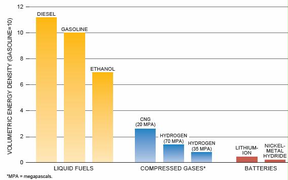
[ Notice how much water biofuels use, especially soybeans for biodiesel
Alice Friedemann www.energyskeptic.com author of “When Trucks Stop Running: Energy and the Future of Transportation”, 2015, Springer]
Notes from “Working Document of the NPC Future Transportation Fuels Study. Topic Paper #31 Water Usage“. July 17, 2012 by John Wind and Ray Dums, 21 pages.
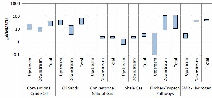
Figure 3. Well-to-Tank (WTT) Hydrocarbon Transportation Fuel Pathways – Fresh Water Consumption (Gal/MMBTU)
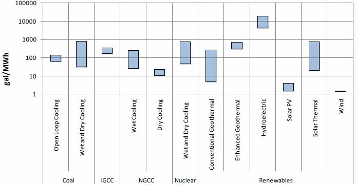
Figure 4. Power Generation Pathways – Life Cycle Water Consumption (gal/MWh)
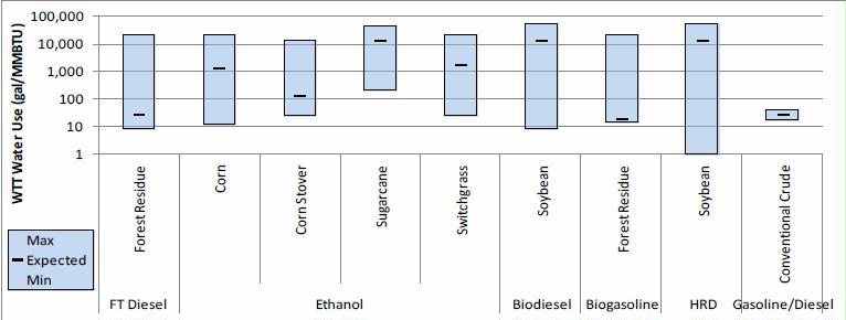
Figure 6. Well-to–Tank (WTT) Water Consumption for Various Biofuel Pathways
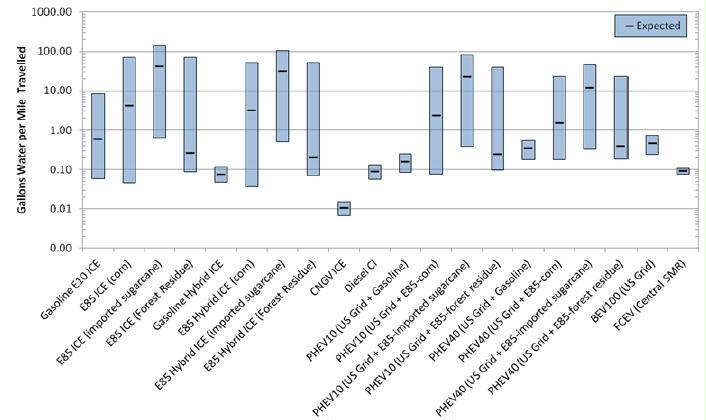
Figure 7. Well-to-Wheels (WTW) Water Consumption for Fuel-Vehicle Systems
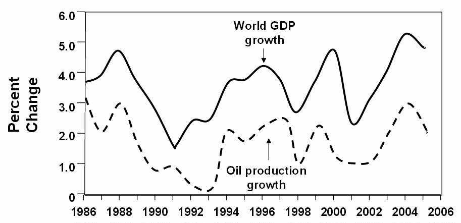
Water is used in significant quantities for producing energy. It is an essential part of the fuel lifecycle, from feedstock production to conversion to final fuels and power. Because water is a limited resource essential for sustaining life, an understanding of water requirements for different fuel options is required. In order to understand the relative impacts of water use in the production of transportation fuels, it is first important to place this use within the context of total global and U.S. water supply and dispositions.
Water resource use is generally described by two measures: volumes withdrawn and volumes consumed.
Water consumption, a subset of total water withdrawn, is the more appropriate measure for resource utilization as this represents water that is removed from the watershed and thus made unavailable for future use. Consumption happens when water evaporates or is contaminated to the point of being unusable. In industrial and thermo-electric applications, for example, this is typically due to evaporative losses in cooling processes. Waste water discharges of fresh water to oceans or disposal to saline aquifers also represent losses of water from a watershed because the freshwater is no longer available for use.
In addition to quantifying volumes of water, the quality of water is an important concern. Fresh water is the most significant since it represents a small fraction of the total global water resource and is critical for sustaining life. Processes that consume fresh water are highly scrutinized and must be evaluated to determine if the use of water resources is prudent.
Figure 1 provides the breakdown between fresh water withdrawn and consumed in the U.S., along with primary end users of that water. In total, approximately 100 billion gallons of fresh water is consumed per day, whereas the total withdrawals are 345 billion gallons per day.
Irrigation for agriculture is the dominant consumer of fresh water in the U.S.
Thermo-electric power generation withdraws about a third but consumes less than a 20th of water resource.
Industrial processes and mining, which includes extraction and processing of fossil hydrocarbon fuels, account for a small fraction of fresh water use.
Freshwater Withdrawals/Consumption (2005 data)
- Domestic 1%/7% Public Supply 13% Thermoelectric 41%/4% Irrigation 37%/81%
- Mining 1%/1% Industrial 5%/3% Aquaculture 3% Livestock 1%/3%
Figure 1. U.S. Freshwater Withdrawals and consumption. Source: USDOE, Energy Demands on Water Resources. Report to Congress on the Interdependency of Energy and Water, 2006. http://pubs.usgs.gov/circ/1344/pdf/c1344.pdf Kenny, J.F., et al. Estimated Use of Water in the United States in 2005. Circular 1344. USGS, U.S. Department of the Interior. Reston, Virginia. 2009. 2 Wu, Consumptive Water Use in the Production of Ethanol and Petroleum Gasoline, Argonne National Laboratory, 2009. ANL/ESD/09–1
Fossil Fuels
Water use associated with transportation fuel production varies greatly between fuel types and is dependent upon the method of extraction and refining. Crude to fuel pathways discussed here include the refining of crudes from conventional, water flood, CO2 flood, and steam flood recovery mechanisms.
Pathways using unconventional resources are oil sands (in situ and mining) and the FT (Fischer–Tropsch) coal-to-liquids and gas-to-liquids processes. Literature values for the water use in gallons per MMBTU fuel produced are given as ranges for each pathway and pathway components (upstream versus downstream). In this report, upstream denotes all processes prior to refining and/or conversion, and downstream denotes processes from refining to distribution. Upstream processes consume more water than their downstream counterparts in the crude oil pathways. All pathways are shown in Figure 3.
Care must be taken when interpreting the water consumption ranges for the different pathways. The broad ranges can be based on regional differences in reservoir characteristics and how the water is recycled, re-used, or treated. Moreover, oil and gas field production characteristics change significantly over time, so the water requirements for a given production technology depend on the site–specific reservoir characteristics, which are a function of the age and production history of the field.
Crude Oil and Natural Gas Pathways
Petroleum extraction consumes relatively little fresh water. Fresh water is used for well construction processes such as drilling and completion in oil and gas resource development. Primary oil and natural gas production, which uses natural reservoir pressure to flow fluids to the wellbore, requires little water.
Secondary methods of recovery, such as water flooding, require increasing amounts, as fresh water may sometimes be required to augment the volume of saline produced water that is re– injected back into the reservoir for pressure support. According to a study of U.S. oil production, the majority of the produced water (approximately 70%), is re–injected to maintain reservoir pressures. The remainder is either cleaned and discharged, or injected into disposal wells.3
Enhanced oil recovery (EOR) methods, such as CO2 or steam injection consume varying amounts of fresh water depending on the process.
Unconventional sources of petroleum such as Canadian oil sands consume varying amounts of water depending on the recovery process. A recent analysis estimates the range of well-to- tank fresh water consumption for crude oil produced onshore in the U.S. is between 22 and 53 gallons per MMBTU, with a technology weighted average of 34 gallons per MMBTU.4 Combining offshore production (as primary recovery with no water consumption) with the onshore production provides a range of fresh water consumption for all U.S. crude oil between 17 and 40 gallons per MMBTU, with a technology weighted average of 27 gallons per MMBTU, including downstream refining.
Crude oil refining consumes fresh water for cooling, boiler feed water, crude desalting, and other processes. This requires refineries to be located in areas with access to stable supplies of water. Refineries typically have extensive water treating facilities and discharge processed/cleaned excess water to surface streams or lakes.
Natural Gas
Conventional natural gas production requires very small (assumed to be negligible) amounts of water for well drilling and completion. Natural gas processing plants use water for cooling and power generation.
The development of shale gas resources requires water for hydraulic fracturing of the shale formations to increase the permeability and enable gas to flow to the producing wells. Over the life of a shale gas well, the water consumption is surprisingly small, though significant volumes are needed over short time periods for hydraulic fracturing. Producers are reusing more of the flow-back water at subsequent fracking sites. The requirements for water quality for the fracture fluids are still being optimized, moving towards higher limits on total dissolved solids (salinity), thus enabling greater reuse of flow-back water. More detail on shale gas production is provided in a recent NPC report.5
Hydrogen from Natural Gas
Natural gas is the feedstock for the primary method of hydrogen production used in petroleum refining, and potentially for use as a transportation fuel. For hydrogen production by steam methane reforming (SMR), the greatest water consumption is in the production of high–pressure steam and, to a lesser extent, the reforming and water gas shift reactions.7 Typically it takes 40-50 gallons of water to produce an MMBTU of H2 fuel. 8,9
Electricity
Thermo-electric generation is one of the major users of fresh water in the U.S. Although it comprises over 33% of all water withdrawals, it only accounts for 4% of fresh water consumption
Biofuels
The United States’ Renewable Fuels Standard (RFS) mandates significantly increased production and use of first-generation and advanced biofuels. Water is intimately tied to the major components of the biofuel production chain –used directly during feedstock production and conversion, and impacted by erosion, runoff, and industrial discharges. Existing demands and impacts on fresh water resources will be increased by the biofuel production mandated by the RFS.
The projected increase in production of biofuel feedstocks between 2006 and 2030 is expected to result in an additional 6.4 billion gallons per day of water withdrawals in the United States. Associated with this withdrawal will be an increase of 5.2 billion gallons per day of water consumption, an increase of over 5% from current total U.S. water consumption (see Figure 1). Compared to the water needed to grow the feedstock, water withdrawals and consumption related to feedstock processing are minor, as they increase from 0.09 to 0.5 and from 0.07 to 0.4 billion gallons per day, respectively.20 Water consumption increases will vary by region and may represent a significant impact on water supplies in areas that are already water-supply stressed.
Biofuel Consumptive Water Use
Water consumption in the biofuel value chain is caused by evaporated and transpired irrigation water, pollution, and water lost during industrial processes within biorefineries. Evaporation during cooling is the primary source of water consumption in biorefining. Water use in biorefineries may also include feedstock cleaning, fermentation, and other processes. A typical biofuel water balance is shown in Figure 5.
Feedstock Production
With the complete implementation of RFS2 in 2022, cellulosic feedstock and corn production for biofuel is expected to approximately double water use compared with biofuel water use in 2006. The increase is likely to be caused by the future production and processing of cellulosic feedstocks.
Corn ethanol production is not likely to contribute to the increased water demands as most corn acreage that would be brought into production for ethanol is already irrigated for other uses. Any feedstock (cellulosic biomass or corn) which is dependent on precipitation rather than irrigation will be advantaged from a water resources perspective.23
Production of the same feedstock in different climates results in a range of water consumption profile values for each crop. For example, water consumption for corn production in three areas of the Midwest with different water balances is shown in Table 2.24 In production regions that are more arid, farmers rely more on irrigation.
Though precipitation is not the only determining variable, this general relationship between precipitation and irrigation requirements applies to most crops.
Table 2. Precipitation and Irrigation Needs (Wu 2009)
Region Precipitation ……..Irrigation
………………………………(inches)……… (gal per MMBTU Ethanol)
- Lower Midwest…. .. 37.8..…………. 93
- Upper Midwest… ….29.5….……… 183
- Western Midwest ..21.7…….. 4,218
Thermo-chemical and biodiesel conversion pathways have lower water requirements than fermentation pathways. The FAME process of biodiesel production and the hydroprocessing of bio-oils require very small water inputs due to the nature of the conversion processes.
Water Consumption Ranges for Selected Biofuel Pathways
While the amount of water (precipitation and irrigation) needed to grow biomass feedstocks dwarfs the amount of water used during conversion, certain feedstocks do not require irrigation (i.e., forest residues and dedicated feedstocks grown in regions with enough precipitation to meet the demands of growth). In these instances, the biomass conversion component of the value chain will be the dominant factor in determining total water consumption.
Water Availability
Biofuel production will have to compete with industrial and power generation requirements, municipalities, and other demands for limited water resources. In general, surface and ground water resources experience regional pressure in most areas of intensive agriculture in the U.S.32 Since annual precipitation and groundwater recharge are finite in all places, increased agricultural consumption associated with feedstock production should be carefully evaluated. Water withdrawals and environmental discharges associated with biorefineries should also be considered. Geographies with stressed water resources can be severely impacted if total water requirements are not thoughtfully considered. Nebraska, Kansas, Colorado, Texas, the Dakotas, eastern Washington and Oregon have stressed or unbalanced water resources (more consumption than recharge) and rely primarily on irrigation for crop production. During periods of drought in any geography, biofuel crops require additional irrigation support to maintain yields. Depleted water resources (Ogallala aquifer, etc.) may not satisfy demand, which will limit the productivity a and sustainability of biofuel production.33
FROM OTHER SOURCES: ENERGY USED IN DRINKING AND SEWAGE TREATMENT
According to the Electric Power Research Institute (EPRI), 4% of America’s electricity is used on drinking water and sewer treatment facilities. In the past, gravity moved water and sewage. Our modern systems use so much energy because 85% of the electricity goes to the pumps that lift and move water and sewage along, often upwards against the flow of gravity, especially in cities that use groundwater. Although the initial groundwater may be shallow, over time as typical unsustainable use grows, the wells need to be drilled deeper and deeper, requiring more and more electricity to pump up.
The most extreme example of this is California’s pumping of water 2,000 feet up from the central valley over the Tehachapi mountains, perhaps the most energy-intensive water supply in the world, and uses 20% of all of California’s electricity generation to do so.
Electricity is also needed to pressurize water to get it to flow through a massive underground pipe network at pressures high enough to guarantee the water will flow to faucets on higher floors of buildings and be strong enough to fight fires. In the past, water flowed out at street level to shared fountains. Since the water infrastructure is falling apart, a great deal of water is lost through leaks, further increasing the amount of electricity that must be used.
Sewage treatment plants are always at the lowest elevations, but even so, electricity is used for pressurized force mains to get sewage over hills, or to flow faster so it doesn’t back up in flat areas.
Climate change in the East and Midwest is likely to cause 30% more sewer overflows and consequent pollution problems.