Notes from 33 page: NREL. 2014. Representation of Solar Capacity Value in the ReEDS Capacity Expansion. National Renewable Energy Laboratory. Technical Report NREL/TP-6A20-61182 March 2014
Comparison of Capacity Value at High Penetration.
Several researchers have conducted modeling efforts to quantify the operational value of solar and other VRRE generation at high (10%+) levels of penetration (Perez, Lew, Mills, Madaeni 2012b, Olson).
These studies find that the capacity credit assigned to solar generation declines significantly at high level of energy penetration. As penetration increases, the marginal economic value of PV drops considerably, primarily because of changes in capacity value, but also in energy value (Mills). Clearly, this decrease in value decreases the overall economics of future solar units (Olson) and could suppress additional investment.
An important emerging issue for electricity system operators is the estimation of renewables’ contributions to reliably meeting system demand, or their capacity value. While the capacity value of thermal generation can be estimated easily, assessment of wind and solar requires a more nuanced approach due to resource variability. Reliability-based methods, particularly assessment of the effective load-carrying capacity (ELCC), are considered to be the most robust and widely accepted techniques for addressing this resource variability. This report validates treatment of solar photovoltaic (PV) capacity value by the Regional Energy Deployment System (ReEDS) capacity expansion model by comparing model results against two sources. The first comparison is against values published by utilities or other entities for known electrical systems at existing solar penetration levels. The second comparison is against a time series ELCC simulation tool for high renewable penetration scenarios in the Western Interconnection. Results from the ReEDS model are found to compare well with both comparisons–despite not being resolved at an hourly scale.
The results are relevant for other capacity-based models that do not use hourly calculations to model solar capacity value. First, solar capacity value should not be parameterized as a static value but must decay with increasing penetration. This is because, for an afternoon-peaking system, as solar penetration increases the system’s peak net load shifts to later in the day– when solar output is lower. Second, long-term planning models should determine how system adequacy requirements differ between time periods in order to approximate loss of load probability (LOLP) calculations. Within the ReEDS model we resolve these issues by using a capacity value estimate that varies by time-slice. Within each time-slice the net load and shadow price on ReEDS’s planning reserve constraint signals the relative importance of additional firm capacity.
An important emerging issue for electricity system operators is the estimation of renewables’ contribution to system adequacy. As supply of electricity must constantly be balanced with demand, system operators typically procure a 10%– 20% capacity reserve margin to meet unplanned outages of existing capacity and unexpected increases in demand (NERC 2013). A generator’s ability to help reliably serve load is measured by its capacity value or effective load carrying capacity (ELCC)—the firm capacity that a generating unit is able to provide during reliability-critical periods. The possibility of outages, whether planned or otherwise, therefore necessitates an accurate and dependable method of assessing each unit’s firm capacity contribution to planning reserves to avoid loss of load. The provision of variable resource renewable energy (VRRE) sources such as wind and solar presents a challenge in the assessment of their contributions to planning reserves. to. Previous studies have estimated the capacity value of photovoltaic (PV) solar (Duignan et al. 2012; Madaeni et al. 2013; Perez et al. 2006), concentrating solar power (CSP) (Madaeni et al. 2012a), and wind (NERC 2013; Keane et al. 2011; Ensslin 2008), finding a wide range of potential capacity values that depend on technology, resource quality, and correlation of generation and demand, among many factors. Numerous techniques can be used to
estimate the capacity value of renewable and conventional generators, though reliability-based methods are considered to be the most robust and widely accepted methods (Madaeni et al. 2013). Reliability-based techniques assess how the addition of a generator affects the overall reliability of the system, specifically, the likelihood of adequately serving load within a planning year. Within this framework, the capacity value of a VRRE source is defined as the maximum additional load that the electrical system could serve while maintaining the same level of reliability or loss of load expectation (LOLE). The amount of additional load that can be served with the addition of the variable generator is its ELCC and is equivalent to its capacity value. A drawback of this method, however, is that it requires extensive data, including time series spanning several years of load and conventional and renewable generation, as well as an inventory of units within a planning area and their respective maintenance schedules and forced outage rates. ELCC-based methods have emerged as an industry-preferred means for assessing the capacity value of generating sources (Milligan and Porter 2008a; NERC 2011; Perez et al. 2008), and a common practice is to maintain an LOLE of 1 day in 10 years or less.
In contrast to reliability-based methods, approximation methods exist that require more modest amounts of system data or that can be performed on generalized systems. Availability of data can particularly be a concern for capacity expansion or capacity planning exercises, which typically are not resolved at the unit or hourly level, but nevertheless require an estimation of VRRE capacity value. One credible method, employed by the Regional Energy Deployment System (ReEDS) model in this report, is the Z-method (Dragoon and Dvortsov 2006), which approximates LOLE through the distribution of a system’s surplus capacity. We supplement the Z-method with a time-period-based method that weighs the relative risk of loss of load within each time period. Utilities and other load-serving entities have historically used a variety of methods to evaluate firm solar capacity. These range from detailed LOLP-based reliability evaluations, to time period-based estimates of solar capacity factors during top-load periods, and even rules of thumb based on engineering judgment (Mills and Wiser 2012). Many utilities do not publically disclose their valuation methodology. There is also uncertainty in characterizing changes in solar capacity value as a function of energy penetration, as there are very few electricity systems with high levels of solar energy penetration to act as case studies. Whatever their method, the assignment of capacity credits to VRRE sources is a part of recognizing and evaluating their economic value (Borenstein 2008)—and therefore becomes increasingly important for justifying their expanded use.
Report Outline. The purpose of this report is two-fold: first, to compare solar capacity values modeled by the ReEDS model to other values published in literature, both at low and high levels of penetration. Second, to understand how such factors as resource quality, energy penetration, and coincidence of generation and load profile determine the modeled capacity value of utility- scale solar. Because contributions to system adequacy increase the value of PV capacity to system operators and power producers, a predictive understanding of how capacity value evolves is an important prerequisite to understanding PV value.
Sensitivity of Capacity Value to Resource Quality. While system operators maintain additional firm capacity beyond expected peak load to hedge against unexpected demand or system contingencies, in reality, there are only a few hours of the year when system adequacy is a truly pressing concern. The capacity value of a generator is assessed based on its ability to serve load during these times, when the LOLP is greatest. Most electrical systems in the United States are summer-peaking, due to cooling loads. As a result, these ‘reliability-critical’ periods typically occur during summer afternoons, though there are also electrical systems that experience peak demand in the winter, when electrical demand is driven by heating loads.
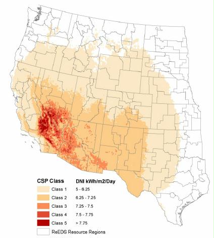
Physical location of a solar unit affects the capacity value of a PV unit at a very basic level. Namely, there is geographic variation in the annual quantity of solar irradiance as well as the diurnal and annual variability in irradiance. Within the ReEDS model, national solar resource is represented at the 134 areas that also serve as load balancing areas (BA). These balancing areas do not necessarily reflect the actual territories of real-world BAs, or specific reliability rules for individual balancing areas.
Nevertheless, this level of geographic detail enables the model to account for geospatial differences in resource quality (Figure 1)—particularly statistical availability during reliability-critical periods. Figure 1: Mean
Correlation of Load and Solar Generation. As a subtler point, geography influences the cooling and heating loads within a balancing area (BA), which thereby influences the timing of high LOLP hours. The key issue is to understand the degree of correlation between a solar unit’s availability and periods of high LOLP. In general, the correlation of load and solar generation varies enough between BA to warrant detailed investigation.
Solar Energy Penetration. Solar PV capacity value is also known to be highly sensitive to increasing levels of PV deployment within the planning region (Perez et al. 2006; Lew et al 2010; Mills & Wiser 2012; Madaeni et al. 2012b; Olson & Jones 2012). PV capacity value is mainly driven by its generation level during the most critical hours of the year, when load is most likely to be dropped due to outages or available capacity. Typically, these periods of time are found during the early evenings of a few weeks of the year, especially for summer-peaking systems. When deployment of PV is at low levels of energy penetration, the additional PV generation does not significantly affect timing of reliability-critical hours. However, since the profile of solar generation is largely coincident with a summer-peaking utility’s load profile, increasing levels of solar generation shifts the critical hours to later hours, when solar irradiance is lower as the sun is setting, decreasing PV capacity value. At high levels of penetration, when net load has been shifted 2 – 3 hours, the capacity factor reaches near-zero levels—as irradiance during the evening is negligible. The most critical hours are typically those with highest levels of net load, i.e., load minus variable generation.
To better illustrate the sensitivity of solar capacity value to energy penetration, the capacity factor is modeled for a representative solar unit in the ReEDS ‘p28’ BA, which overlaps with territory served by the Arizona Public Service utility in central Arizona. Demand in this BA is summer-peaking and the top load hours typically occur during late August afternoons.
As levels of annual solar energy penetration increase from 0% to 20%, the peak load in the diurnal load profile is reduced and shifted to later in the day (Figures 2 and 3). The capacity factor at the point of peak net load erodes following an exponential form and, as predicted, becomes negligible at high levels of annual energy penetration.
In particular, the model uses a high level of spatial resolution—where wind and CSP resources are defined at 356 resource regions and solar PV at the 134 regions that also serve as load BAs. Each resource is regionally characterized by a set of supply curves—constructed from NREL resource assessments (Lopez et al. 2012)—that distinguish resource quality and the cost of accessing the local transmission network. This level of geographic detail enables the model to account for geospatial differences in resource quality, transmission needs, electrical (grid-related) boundaries, political and jurisdictional boundaries, and demographic distributions.
The 134 load regions are connected by an aggregated transmission network that gives ReEDS the ability to discern the relative value of development sites across regions.
For new investments, ReEDS can choose from a broad portfolio of conventional generation, renewable generation, storage, and demand-side technologies. Plants provide power to meet load, capacity toward adequacy requirements, and operating (spinning or non-spinning) reserves. Conventional generators contribute their nameplate capacity toward adequacy requirements and supply operating reserves while variable renewables contribute their calculated capacity value and require additional operating reserves.
Three solar PV system types are modeled—utility-scale (UPV), distributed utility-scale (DUPV), and distributed rooftop. UPV and DUPV are interconnected to the grid at the transmission level and are assumed to be utility controlled, whereas distributed rooftop is connected at the distribution network level, behind the meter. Rooftop PV projections are developed outside of ReEDS, in NREL’s SolarDS model (Denholm et al. 2009) because decisions on rooftop installations are assumed to be made on a different basis (i.e., by individuals) than centralized utility or power-producer decisions. The differences in ReEDS between UPV and DUPV are primarily about size and siting freedom: DUPV systems are smaller and are assumed to be close to load, while UPV systems are wide-ranging. This report exclusively applies to UPV and does not analyze capacity value for DUPV and rooftop PV systems.
UPV represents single-axis tracking PV systems with a unit size of 100 MW.
The ReEDS transmission network is a 134-node system connected by roughly 300 transmission corridors representing the collection of real transmission lines that cross BA boundaries and are characterized by the carrying capacity of those lines.
Capacity Value Calculations. ReEDS uses a measure of a VRRE generator’s ELCC to determine its contributions to planning reserves in each of the 17 time periods. That is, adequacy/reliability is defined in terms of the likelihood that the system (BA, transmission zone, service territory) will have insufficient available generating capacity to meet load during a given period.
The Z-method is used by ReEDS to estimate capacity value because it permits the approximation of capacity value without conducting an hourly time-series analysis, which is infeasible given ReEDS’s temporal resolution. However, the Z-method assumption of a Gaussian form can be violated under high-renewable scenarios if the real time-slice probability distribution of VRRE output does not follow a Gaussian distribution.
ReEDS Scenario Parameters. ReEDS calculations of solar capacity value were compared to the studies in Table 1 in order to benchmark performance of the model. To facilitate an equitable comparison, scenarios were constructed to match each utility region’s geographic location, existing generation fleet, and PV deployment levels as closely as possible. By default, ReEDS uses historic capacity expansion from 2010 to 2013 and business-as-usual assumptions for capacity expansion projections thereafter.
Figure 6. Comparison of solar capacity values in reliability-critical time periods to published values
Unfortunately, there are very few actual electrical systems operating at high levels of solar penetration, and so there is scarce available literature on the capacity value of solar on real electrical systems.
Figure 7. State-based solar PV capacity values for reliability-critical time periods for WWSIS-2 scenarios in 2020
Notice, also, that there is some erosion of capacity value within a time-slice as penetration increases. This is consistent with the hypothesis that within any set region adding more PV increases its self-correlation. As does a system operator, ReEDS has the capability to diversify its resource base somewhat, but not fully, and the intra-time-slice erosion represents the limit of that ability.
We suggest that capacity value erosion within a time period is explained through increased self-correlation of energy production, as well as decreases in available high-quality resource sites within the region.
Conclusion.
ReEDS was designed to represent characteristics that drive variation in investment and operation costs of renewable energy technologies, including geospatial resource assessment and integration of variable resources into a reliable electricity grid. Because these characteristics give the model accurate information about the economic value of, for instance, an additional unit of solar capacity, ReEDS is able to make well-informed investment decisions. Capacity value, as discussed here, is one of the economic components ReEDS includes in its decision making—one that can change dramatically with system configuration and is important to model dynamically.
To accurately reflect solar capacity value in capacity expansion decisions, ReEDS models a number of factors that determine its ELCC. These include representation of the statistical availability of a solar unit, a high level of geographic resolution in resource quality and grid conditions, and correlation of residual load and solar generation. Additionally, ReEDS simultaneously considers adequacy issues in all time-slices. Because the value of capacity services is highest during reliability-critical periods, and increased solar generation shifts those periods away from peak solar output, this accounts for the diminishing capacity value of solar at high levels of penetration. We find that capacity value outcomes from the ReEDS model compare favorably with results from hourly resolution ELCC-based analyses for a range of real and modeled levels of solar energy penetration.
References
Amelin, M. (May 2009). “Comparison of Capacity Credit Calculation Methods for Conventional Power Plants and Wind Power.” IEEE Transactions on Power Systems (24:2); pp. 685–691.
Borenstein, S. (January 2008). “The Market Value and Cost of Solar Photovoltaic Electricity Production.” UC Berkeley: Center for the Study of Energy Markets. Berkeley, CA: UC Berkeley
Bialek, J. (1996). “Tracing the Flow of Electricity in Generation, Transmission and Distribution.” IEEE Proceedings (143: 4); pp. 313-320).
Billinton, R.; Allan, R.N. (1996). Reliability Evaluation of Power Systems. New York, NY: Plenum Press.
Denholm, P.; Drury, E.; Margolis, R. (September 2009). The Solar Deployment System (SolarDS) Model: Documentation and Sample Results. NREL/TP-6A2-45832. Golden, CO: National Renewable Energy Laboratory, 52 pp.
Dragoon, K.; Dvortsov, V. (2006). “Z-Method for Power System Resource Adequacy Applications.” IEEE Transactions on Power Systems (21:2); pp. 982-988.
Duignan, R.; Dent, C.; Mills, A.; Samaan, N.; Milligan, M.; Keane, A.; O’Malley, M. (2012). “Capacity Value of Solar Power.” Power and Energy Society, IEEE General Meeting; 6 pp.
EIA. (2013). Annual Energy Outlook 2013. DOE/EIA-0383. Washington, DC: EIA.
Ibanez, E.; Milligan, M. (September 2012). “A Probabilistic Approach to Quantifying the Contribution of Variable Generation and Transmission to System Reliability.” NREL/CP-5500-56219. Golden, CO: National Renewable Energy Laboratory.
Integration of Variable Generation Task Force. (2011). “Methods to Model and Calculate Capacity Contributions of Variable Generation for Resource Adequacy Planning.” Princeton, NJ: North American Electric Reliability Corporation. Accessed January 27, 2014: http://www.nerc.com/docs/pc/ivgtf/IVGTF1-2.pdf.
Keane, A.; Milligan, M; Dent, C; Hasche, B.; D’Annunzio, C; Dragoon, K.; Holttinen, H.; Samaan, N.; S¨oder, L.; O’Malley, M. (May 2011). “Capacity Value of Wind Power.” IEEE Transactions on Power Systems (26:2); pp. 564–572.
Lew, D.; Brinkman, G.; Ibanez, E.; Florita, A.; Heaney, M.; Hodge, B.; Hummon, M.; Stark, G.; King, J.; Lefton, S.; Kumar, N.; Agan, D.; Jordan, G.; Venkataraman, S. (2013). Western Wind and Solar Integration Study: Phase 2. TP-5500-55588. Golden, CO: National Renewable Energy Laboratory, 244 pp. Accessed January 27, 2014: http://www.nrel.gov/docs/fy13osti/55588.pdf.
Lopez, A.; Roberts, B.; Heimiller, D.; Blair, N.; Porro, G. (2012). U.S. Renewable Energy Technical Potentials: A GIS-Based Analysis. TP-6A20-51946. Golden, CO: National Renewable Energy Laboratory, 40 pp. Accessed January 27, 2014: http://www.nrel.gov/docs/fy12osti/51946.pdf.
Lu, S.; Diao, R.; Samaan, N.; Etinov, P. (2012). “Capacity Value of PV and Wind Generation in the NV Energy System.” PNNL-22117. Richland, WA: Pacific Northwest National Laboratory, 35 pp.
Madaeni, S.H.; Sioshansi, R.; Denholm, P. (July 2012a) “The Capacity Value of Solar Generation in the Western United States.” Power and Energy Society General Meeting. IEEE, pp.1-8, 22-26 July 2012. doi: 10.1109/PESGM.2012.6345521.
Madaeni, S.H.; Sioshansi, R.; Denholm, P. (May 2012b). “Estimating the Capacity Value of Concentrating Solar Power Plants: A Case Study of the Southwestern United States.” IEEE Transactions on Power Systems (27:2); pp. 1116–1124.
Madaeni, S. H.; Sioshansi, R.; Denholm, P. (2013). “Comparison of Capacity Value Estimation Techniques for Photovoltaic Solar Power.” IEEE Journal of Photovoltaics (3:1); pp. 407-415.
Milligan, M.; Porter, K. (2008a) “Determining the Capacity Value of Wind: An Updated Survey of Methods and Implementation”. NREL/CP-500-43433. Golden, CO: National Renewable Energy Laboratory, June 2008. http://www.nrel.gov/docs/fy08osti/43433.pdf.
Milligan, M.; Porter, K. (2008b). “Wind Capacity Credit in the United States.” In Proc. IEEE Power and Energy Society Gral. Meeting, pp. 1-5.
Milligan, M. (2002). “A Chronological Reliability Model Incorporating Wind Forecasts to Assess Wind Plant Reserve Allocation.” Golden, CO: National Renewable Energy Laboratory. Accessed January 27, 2014: http://www.nrel.gov/docs/fy02osti/32210.pdf.
Mills, A.; Wiser, R. (2012). “An Evaluation of Solar Valuation Methods Used in Utility Planning and Procurement Processes.” LBNL-5933E. Berkeley, CA: Lawrence Berkeley National Laboratory.
NERC. (December 2013). “2013 Long-Tern Reliability Assessment.” Princeton, NJ: North American Electric Reliability Corp.
NERC. (March 2011). “Methods to Model and Calculate Capacity Contributions of Variable Generation for Resource Adequacy Planning.” Princeton, NJ: North American Electric Reliability Corp.
National Renewable Energy Laboratory (NREL). (2010a). “System Advisor Model (SAM) Version 2010.4.12.” Accessed April 12, 2010: https://www.nrel.gov/analysis/sam/.
(NREL). (2012). Renewable Electricity Futures Study. Hand, M.M.; Baldwin, S.; DeMeo, E.; Reilly, J.M.; Mai, T.; Arent, D.; Porro, G.; Meshek, M.; Sandor, D. eds. 4 vols. NREL/TP-6A20-52409. Golden, CO: National Renewable Energy Laboratory.
National Solar Radiation Database. (2010). “National Solar Radiation Data Base 1991 – 2010 Update.” Accessed November 11, 2013: http://rredc.nrel.gov/solar/old_data/nsrdb/1991-2010/.
Orwig, K.; Hummon, M.; Hodge, B.-M.; Lew, D. (2011). “Solar Data Inputs for Integration and Transmission Planning Studies.” Proc. 1st Int. Workshop on Integration of Solar Power into Power Systems, Aarhu, Denmark, October 2011.
Perez, R.; Taylor, M.; Hoff, T.; Ross, J.P. (2008). “Reaching Consensus in the Definition of Photovoltaics Capacity Credit in the USA: A Practical Application of Satellite-Derived Solar Resource Data.” IEEE Journal of Selected Topics in Applied Earth Observations and Remote Sensing (1:1); pp 28–33.
Perez, R.; Hoff, T.E. (2008). “Energy and Capacity Valuation of Photovoltaic Power Generation in New York.” Solar Alliance and the New York Solar Energy Industry Association, March 2008. Accessed January 27, 2014: http://asrc.albany.edu/people/faculty/perez/publications/Utility%20Peak%20Shaving%20and%20Capacity%20Credit/Papers%20on%20PV%20Load%20Matching%20and%20Economic%20Evaluation/Energy%20Capacity%20Valuation-08.pdf.
Perez, R; Margolis, R.; Kmiecik, M; Schwab, M.; Perez, M. (June 2006). Update: Effective Load-Carrying Capability of Photovoltaics in the United States. NREL/CP-620-40068. Golden, CO: National Renewable Energy Laboratory.
Public Service Company of New Mexico. (July 2011). “Electric Integrated Resource Plan: 2011-2030.” Accessed January 27, 2014: http://www.pnm.com/regulatory/pdf_electricity/irp_2011-2030.pdf.
Renewable Electricity Futures Study. (2012). Golden, CO: National Renewable Energy Laboratory; NREL Report No. TP-6A20-52409.
R.W. Beck, Inc. (January 2009). “Distributed Renewable Energy Operating Impacts and Valuation Study: Prepare for Arizona Public Service.” 424 pp.
Saha, A. (12 April 2013). “Review of Coal Plant Retirements.” M.J. Bradley & Associates.
SAIC Energy, Environment, & Infrastructure LLC. (May 2013). “2013 Updated Solar PV Value Report.” Arizona Public Service. Accessed January 27, 2014: http://www.solarfuturearizona.com/2013SolarValueStudy.pdf.
Short, W.; Sullivan, P.; Mai, T.; Mowers, M.; Uriate, C.; Blair, N.; Heimiller, D.; Martinez, A. (2011). “Regional Energy Deployment System (ReEDS).” TP-6A20-46534. Golden, CO: National Renewable Energy Laboratory, 94 pp.
Stott, B.; Jardim, J.; Alsac, O. (August 2009). “DC Power Flow Revisited.” IEEE Transactions on Power Systems (24:3). Accessed January 27, 2014: http://ieeexplore.ieee.org/stamp/stamp.jsp?tp=&arnumber=4956966&tag=1. EERE. (February 2012). SunShot Vision Study. Energy Efficiency & Renewable Energy (EERE), BK-5200-47927; DOE/GO-102012-3037. 320 pp.; 3TIER. (2010). “Development of Regional Wind Resource and Wind Plant Output Datasets.” NREL/SR-550-47676. Golden, CO: National Renewable Energy Laboratory. Accessed January 27, 2014: http://www.nrel.gov/docs/fy10osti/47676.pdf.
Tri-State Generation and Transmission Association, Inc. (November 2010). “Integrated Resource Plan/ Electric Resource Plan for Tri-State Generation and Transmission Association Inc.” Accessed January 27, 2014: http://www.tristategt.org/ResourcePlanning/documents/Tri-State_IRP-ERP_Final.pdf.
Ventyx. (2010). “Energy Market Data.” Accessed January 27, 2014: http://www.ventyx.com/velocity/energy-market-data.asp.
Western Electricity Coordinating Council. (2009). “Transmission Expansion Planning Policy Committee 2009 Study Program Results Report.” Accessed January 27, 2014: www.wecc.biz/committees/ BOD/TEPPC/Shared Documents/TEPPC Annual Reports.
Wilcox, S; Anderberg, M; George, R; Marion, W; Myers, D; Renne, D; Lott, N; Whitehurst, T; Beckman, W; Gueymard, C; Perez, R; Stackhouse, P.; Vignola, F. (July 2007). “Completing Production of the Updated National Solar Radiation Database for the United States.” CP‐581‐41511. Golden, CO: National Renewable Energy Laboratory.
Xcel Energy Services, Inc. (May 2013). “Costs and Benefits of Distributed Solar Generation on the Public Service Company of Colorado System.”