Gail Tverberg: 8 pitfalls in evaluating green energy solutions

Eight Pitfalls in Evaluating Green Energy Solutions

Does the recent climate accord between US and China mean that many countries will now forge ahead with renewables and other green solutions? I think that there are more pitfalls than many realize.

Pitfall 1. Green solutions tend to push us from one set of resources that are a problem today (fossil fuels) to other resources that are likely to be problems in the longer term.  

The name of the game is “kicking the can down the road a little.” In a finite world, we are reaching many limits besides fossil fuels:

  1. Soil quality–erosion of topsoil, depleted minerals, added salt
  2. Fresh water–depletion of aquifers that only replenish over thousands of years
  3. Deforestation–cutting down trees faster than they regrow
  4. Ore quality–depletion of high quality ores, leaving us with low quality ores
  5. Extinction of other species–as we build more structures and disturb more land, we remove habitat that other species use, or pollute it
  6. Pollution–many types: CO2, heavy metals, noise, smog, fine particles, radiation, etc.
  7. Arable land per person, as population continues to rise

The danger in almost every “solution” is that we simply transfer our problems from one area to another. Growing corn for ethanol can be a problem for soil quality (erosion of topsoil), fresh water (using water from aquifers in Nebraska, Colorado). If farmers switch to no-till farming to prevent the erosion issue, then great amounts of Round Up are often used, leading to loss of lives of other species.

Encouraging use of forest products because they are renewable can lead to loss of forest cover, as more trees are made into wood chips. There can even be a roundabout reason for loss of forest cover: if high-cost renewables indirectly make citizens poorer, citizens may save money on fuel by illegally cutting down trees.

High tech goods tend to use considerable quantities of rare minerals, many of which are quite polluting if they are released into the environment where we work or live. This is a problem both for extraction and for long-term disposal.

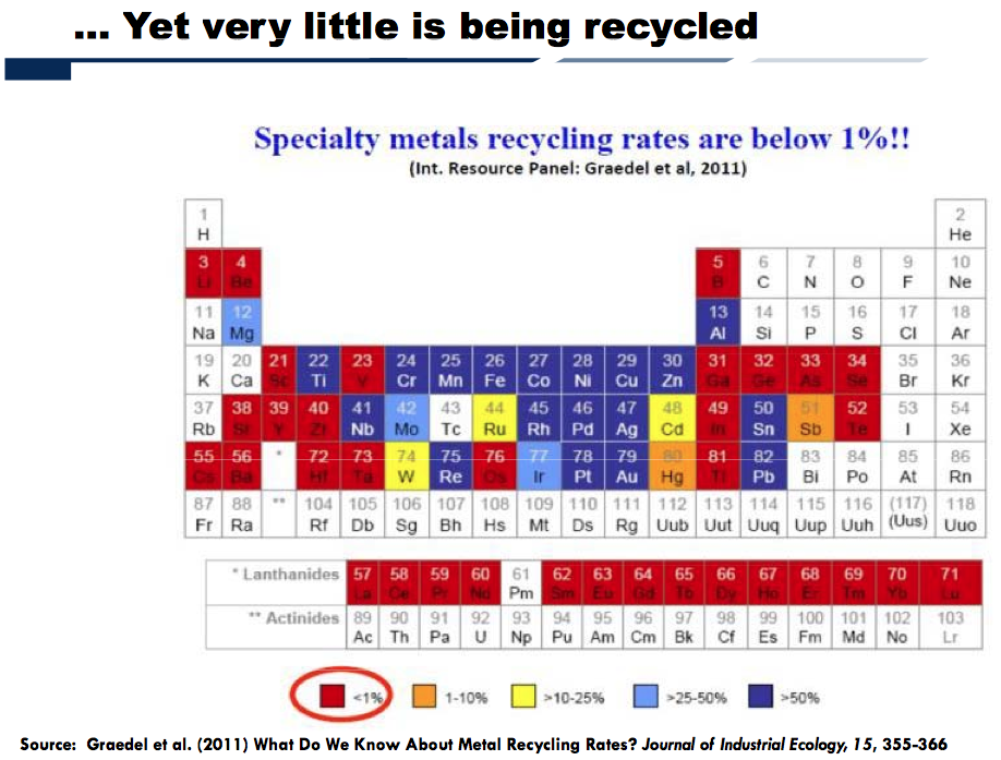
Pitfall 2. Green solutions that use rare minerals are likely not very scalable because of quantity limits and low recycling rates.  

Computers, which are the heart of many high-tech goods, use almost the entire periodic table of elements.

Figure 1. Slide by Alicia Valero showing that almost the entire periodic table of elements is used for computers.

When minerals are used in small quantities, especially when they are used in conjunction with many other minerals, they become virtually impossible to recycle. Experience indicates that less than 1% of specialty metals are recycled.

Figure 2. Slide by Alicia Valero showing recycling rates of elements.

Green technologies, including solar panels, wind turbines, and batteries, have pushed resource use toward minerals that were little exploited in the past. If we try to ramp up usage, current mines are likely to deplete rapidly. We will eventually need to add new mines in areas where resource quality is lower and concern about pollution is higher. Costs will be much higher in such mines, making devices using such minerals less affordable, rather than more affordable, in the long run.

Of course, a second issue in the scalability of these resources has to do with limits on oil supply. As ores of scarce minerals deplete, more rather than less oil will be needed for extraction. If oil is in short supply, obtaining this oil is also likely to be a problem, also inhibiting scalability of the scarce mineral extraction. The issue with respect to oil supply may not be high price; it may be low price, for reasons I will explain later in this post.

Pitfall 3. High-cost energy sources are the opposite of the “gift that keeps on giving.” Instead, they often represent the “subsidy that keeps on taking.”

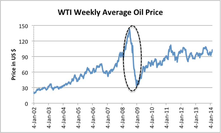
Oil that was cheap to extract (say $20 barrel) was the true “gift that keeps on giving.” It made workers more efficient in their jobs, thereby contributing to efficiency gains. It made countries using the oil more able to create goods and services cheaply, thus helping them compete better against other countries. Wages tended to rise, as long at the price of oil stayed below $40 or $50 per barrel (Figure 3).

Figure 3. Average wages in 2012$ compared to Brent oil price, also in 2012$. Average wages are total wages based on BEA data adjusted by the CPI-Urban, divided total population. Thus, they reflect changes in the proportion of population employed as well as wage levels.

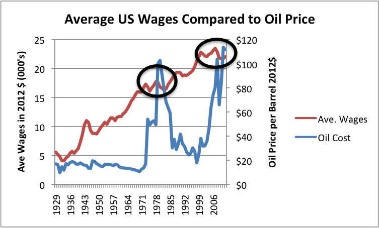
More workers joined the work force, as well. This was possible in part because fossil fuels made contraceptives available, reducing family size. Fossil fuels also made tools such as dishwashers, clothes washers, and clothes dryers available, reducing the hours needed in housework. Once oil became high-priced (that is, over $40 or $50 per barrel), its favorable impact on wage growth disappeared.

When we attempt to add new higher-cost sources of energy, whether they are high-cost oil or high-cost renewables, they present a drag on the economy for three reasons:

  1. Consumers tend to cut back on discretionary expenditures, because energy products (including food, which is made oil and other energy products) are a necessity. These cutbacks feed back through the economy and lead to layoffs in discretionary sectors. If they are severe enough, they can lead to debt defaults as well, because laid-off workers have difficulty paying their bills.
  2.  An economy with high-priced sources of energy becomes less competitive in the world economy, competing with countries using less expensive sources of fuel. This tends to lead to lower employment in countries whose mix of energy is weighted toward high-priced fuels.
  3. With (1) and (2) happening, economic growth slows. There are fewer jobs and debt becomes harder to repay.

In some sense, the cost producing of an energy product is a measure of diminishing returns–that is, cost is a measure of the amount of resources that directly and indirectly or indirectly go into making that device or energy product, with higher cost reflecting increasing effort required to make an energy product. If more resources are used in producing high-cost energy products, fewer resources are available for the rest of the economy. Even if a country tries to hide this situation behind a subsidy, the problem comes back to bite the country. This issue underlies the reason that subsidies tend to “keeping on taking.”

The dollar amount of subsidies is also concerning. Currently, subsidies for renewables (before the multiplier effect) average at least $48 per barrel equivalent of oil.1 With the multiplier effect, the dollar amount of subsidies is likely more than the current cost of oil (about $80), and possibly even more than the peak cost of oil in 2008 (about $147). The subsidy (before multiplier effect) per metric ton of oil equivalent amounts to $351. This is far more than the charge for any carbon tax.

Pitfall 4. Green technology (including renewables) can only be add-ons to the fossil fuel system.

A major reason why green technology can only be add-ons to the fossil fuel system relates to Pitfalls 1 through 3. New devices, such as wind turbines, solar PV, and electric cars aren’t very scalable because of high required subsidies, depletion issues, pollution issues, and other limits that we don’t often think about.

A related reason is the fact that even if an energy product is “renewable,” it needs long-term maintenance. For example, a wind turbine needs replacement parts from around the world. These are not available without fossil fuels. Any electrical transmission system transporting wind or solar energy will need frequent repairs, also requiring fossil fuels, usually oil (for building roads and for operating repair trucks and helicopters).

Given the problems with scalability, there is no way that all current uses of fossil fuels can all be converted to run on renewables. According to BP data, in 2013 renewable energy (including biofuels and hydroelectric) amounted to only 9.4% of total energy use. Wind amounted to 1.1% of world energy use; solar amounted to 0.2% of world energy use.

Pitfall 5. We can’t expect oil prices to keep rising because of affordability issues.  

Economists tell us that if there are inadequate oil supplies there should be few problems:  higher prices will reduce demand, encourage more oil production, and encourage production of alternatives. Unfortunately, there is also a roundabout way that demand is reduced: wages tend to be affected by high oil prices, because high-priced oil tends to lead to less employment (Figure 3). With wages not rising much, the rate of growth of debt also tends to slow. The result is that products that use oil (such as cars) are less affordable, leading to less demand for oil. This seems to be the issue we are now encountering, with many young people unable to find good-paying jobs.

If oil prices decline, rather than rise, this creates a problem for renewables and other green alternatives, because needed subsidies are likely to rise rather than disappear.

The other issue with falling oil prices is that oil prices quickly become too low for producers. Producers cut back on new development, leading to a decrease in oil supply in a year or two. Renewables and the electric grid need oil for maintenance, so are likely to be affected as well. Related posts include Low Oil Prices: Sign of a Debt Bubble Collapse, Leading to the End of Oil Supply? and Oil Price Slide – No Good Way Out.

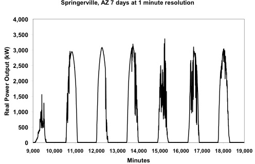
Pitfall 6. It is often difficult to get the finances for an electrical system that uses intermittent renewables to work out well.  

Intermittent renewables, such as electricity from wind, solar PV, and wave energy, tend to work acceptably well, in certain specialized cases:

  • When there is a lot of hydroelectricity nearby to offset shifts in intermittent renewable supply;
  • When the amount added is sufficient small that it has only a small impact on the grid;
  • When the cost of electricity from otherwise available sources, such as burning oil, is very high. This often happens on tropical islands. In such cases, the economy has already adjusted to very high-priced electricity.

Intermittent renewables can also work well supporting tasks that can be intermittent. For example, solar panels can work well for pumping water and for desalination, especially if the alternative is using diesel for fuel.

Where intermittent renewables tend not to work well is when

  1. Consumers and businesses expect to get a big credit for using electricity from intermittent renewables, but
  2. Electricity added to the grid by intermittent renewables leads to little cost savings for electricity providers.

For example, people with solar panels often expect “net metering,” a credit equal to the retail price of electricity for electricity sold to the electric grid. The benefit to electric grid is generally a lot less than the credit for net metering, because the utility still needs to maintain the transmission lines and do many of the functions that it did in the past, such as send out bills. In theory, the utility still should get paid for all of these functions, but doesn’t. Net metering gives way too much credit to those with solar panels, relative to the savings to the electric companies. This approach runs the risk of starving fossil fuel, nuclear, and grid portion of the system of needed revenue.

A similar problem can occur if an electric grid buys wind or solar energy on a preferential basis from commercial providers at wholesale rates in effect for that time of day. This practice tends to lead to a loss of profitability for fossil fuel-based providers of electricity. This is especially the case for natural gas “peaking plants” that normally operate for only a few hours a year, when electricity rates are very high.

Germany has been adding wind and solar, in an attempt to offset reductions in nuclear power production. Germany is now running into difficulty with its pricing approach for renewables. Some of its natural gas providers of electricity have threatened to shut down because they are not making adequate profits with the current pricing plan. Germany also finds itself using more cheap (but polluting) lignite coal, in an attempt to keep total electrical costs within a range customers can afford.

Pitfall 7. Adding intermittent renewables to the electric grid makes the operation of the grid more complex and more difficult to manage. We run the risk of more blackouts and eventual failure of the grid. 

In theory, we can change the electric grid in many ways at once. We can add intermittent renewables, “smart grids,” and “smart appliances” that turn on and off, depending on the needs of the electric grid. We can add the charging of electric automobiles as well. All of these changes add to the complexity of the system. They also increase the vulnerability of the system to hackers.

The usual assumption is that we can step up to the challenge–we can handle this increased complexity. A recent report by The Institution of Engineering and Technology in the UK on the Resilience of the Electricity Infrastructure questions whether this is the case. It says such changes, ” .  .  . vastly increase complexity and require a level of engineering coordination and integration that the current industry structure and market regime does not provide.” Perhaps the system can be changed so that more attention is focused on resilience, but incentives need to be changed to make resilience (and not profit) a top priority. It is doubtful this will happen.

The electric grid has been called the worlds ‘s largest and most complex machine. We “mess with it” at our own risk. Nafeez Ahmed recently published an article called The Coming Blackout Epidemic, discussing challenges grids are now facing. I have written about electric grid problems in the past myself: The US Electric Grid: Will it be Our Undoing?

Pitfall 8. A person needs to be very careful in looking at studies that claim to show favorable performance for intermittent renewables.  

Analysts often overestimate the benefits of wind and solar. Just this week a new report was published saying that the largest solar plant in the world is so far producing only half of the electricity originally anticipated since it opened in February 2014.

In my view, “standard” Energy Returned on Energy Invested (EROEI) and Life Cycle Analysis (LCA) calculations tend to overstate the benefits of intermittent renewables, because they do not include a “time variable,” and because they do not consider the effect of intermittency. More specialized studies that do include these variables show very concerning results. For example, Graham Palmer looks at the dynamic EROEI of solar PV, using batteries (replaced at eight year intervals) to mitigate intermittency.2 He did not include inverters–something that would be needed and would reduce the return further.

Figure 4. Graham Palmer's chart of Dynamic Energy Returned on Energy Invested from "Energy in Australia."

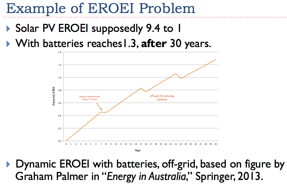
Palmer’s work indicates that because of the big energy investment initially required, the system is left in a deficit energy position for a very long time. The energy that is put into the system is not paid back until 25 years after the system is set up. After the full 30-year lifetime of the solar panel, the system returns 1.3 times the initial direct energy investment.

One further catch is that the energy used in the EROEI calculations includes only a list of direct energy inputs. The total energy required is much higher; it includes indirect inputs that are not directly measured as well as energy needed to provide necessary infrastructure, such as roads and schools. When these are considered, the minimum EROEI needs to be something like 10. Thus, the solar panel plus battery system modeled is really a net energy sink, rather than a net energy producer.  

Another study by Weissbach et al. looks at the impact of adjusting for intermittency. (This study, unlike Palmer’s, doesn’t attempt to adjust for timing differences.) It concludes, “The results show that nuclear, hydro, coal, and natural gas power systems . . . are one order of magnitude more effective than photovoltaics and wind power.”

Conclusion

It would be nice to have a way around limits in a finite world. Unfortunately, this is not possible in the long run. At best, green solutions can help us avoid limits for a little while longer.

The problem we have is that statements about green energy are often overly optimistic. Cost comparisons are often just plain wrong–for example, the supposed near grid parity of solar panels is an “apples to oranges” comparison. An electric utility cannot possibility credit a user with the full retail cost of electricity for the intermittent period it is available, without going broke. Similarly, it is easy to overpay for wind energy, if payments are made based on time-of-day wholesale electricity costs. We will continue to need our fossil-fueled balancing system for the electric grid indefinitely, so we need to continue to financially support this system.

There clearly are some green solutions that will work, at least until the resources needed to produce these solutions are exhausted or other limits are reached. For example, geothermal may be solutions in some locations. Hydroelectric, including “run of the stream” hydro, may be a solution in some locations. In all cases, a clear look at trade-offs needs to be done in advance. New devices, such as gravity powered lamps and solar thermal water heaters, may be helpful especially if they do not use resources in short supply and are not likely to cause pollution problems in the long run.

Expectations for wind and solar PV need to be reduced. Solar PV and offshore wind are both likely net energy sinks because of storage and balancing needs, if they are added to the electric grid in more than very small amounts. Onshore wind is less bad, but it needs to be evaluated closely in each particular location. The need for large subsidies should be a red flag that costs are likely to be high, both short and long term. Another consideration is that wind is likely to have a short lifespan if oil supplies are interrupted, because of its frequent need for replacement parts from around the world.

Some citizens who are concerned about the long-term viability of the electric grid will no doubt want to purchase their own solar systems with inverters and back-up batteries. I see no reason to discourage people who want to do this–the systems may prove to be of assistance to these citizens. But I see no reason to subsidize these purchases, except perhaps in areas (such as tropical islands) where this is the most cost-effective way of producing electric power.

Notes:

[1] In 2013, the total amount of subsidies for renewables was $121 billion according to the IEA. If we compare this to the amount of renewables (biofuels + other renewables) reported by BP, we find that the subsidy per barrel of oil equivalent in was $48 per barrel of oil equivalent. These amounts are likely understated, because BP biofuels include fuel that doesn’t require subsidies, such as waste sawdust burned for electricity.

[2] Palmer’s work is published in Energy in Australia: Peak Oil, Solar Power, and Asia’s Economic Growth, published by Springer in 2014. This book is part of Prof. Charles Hall’s “Briefs in Energy” series.

Posted in Alternative Energy, Gail Tverberg | Tagged , , , , , , , , , | Comments Off on Gail Tverberg: 8 pitfalls in evaluating green energy solutions

Why You Should Love Trains

Why You Should Love Trains

by Alice Friedemann    November 13, 2014

Trains rock!

Trains are over 4 times more fuel efficient than trucks. On average it takes just 1 gallon to move a ton 473 miles, using just 2% of transportation oil. Trucks suck, burning 46% of transportation oil— 20% medium / heavy trucks, and 26% light trucks (FRA, USDOT 2014b, Davis).

Energy has been so cheap and plentiful we’ve blown our oil wad on gas-guzzling trucks, the limousines of the freight world. They lumber over 4 million miles of roads, often half empty with just the parts needed at a factory and drive back empty for their next haul.

A short-sighted transportation policy that favored energy-gulping trucks has reduced our rail system from 380,000 miles of tracks in 1920 to 140,000. About 45,000 of these miles are short-line tracks run by 500 small rail companies that go to grain elevators, steel mills, stock yards, and other businesses. The other 95,000 miles are the mainline tracks that move freight across the country, run by the seven large class 1 rail companies. These tracks tend to be in better condition and capable of hauling heavier railcars and locomotives than short-line rail.

Trains keep lights burning and bread on the table. Half of what trains haul (by weight) is energy related.

Rail excels at hauling heavy goods like coal and grain long distances (615 miles on average), so much so, that when you multiply weight times miles traveled, trains carry 45% of freight by ton-miles, versus 38% for trucks, yet trucks carry most of the weight overall, about three-quarters of it, because most freight travels less than 250 miles (USDOT 2014a).

Almost 40% of all tons carried by trains are coal, 42% of it from Wyoming, and 93% of U.S. coal will be used to generate electricity.

Trains also carry refined petroleum and coke (2.6%), fracked (tight) oil (2.2%), natural gas based fertilizers (2%) and plastics (2%), ethanol (1.5%), and petrochemicals (1%).

Other major commodities trains haul are chemicals 10%, grain 7%, crushed stone, sand, gravel 7%, food 6%, metals 3%, waste & scrap 2%, pulp/paper 2%, lumber/wood 1%, and import/export containers, which could contain just about anything.

Why not build more railroad tracks to conserve oil?

This seems like a no-brainer:

  • Heavy-duty trucks ruin roads and bridges and don’t pay for 20% of the damage (HR). Moving more freight by rail would save billions of dollars in road maintenance, and reduce road congestion (one train equals several hundred trucks), saving $121 billion in wasted fuel and time (TTI).
  • For every 10% of truck freight switched to rail, another billion gallons of fuel are saved as well as reducing nitrous oxides 80%, particulates 90%, and greenhouse gas emissions by 75% per ton-mile (EPA).
  • Railroad tracks are cheaper to add and maintain, $129,000 per mile (including bridges, land, buildings, wharves, docks, etc. (AAR 2012) versus $327,000 per mile to add and maintain roads (average of USDOT 2010-11-12).
  • Maintaining tracks is $10-$14,000 per mile/year (Liu, TDOT). Resurfacing and restoring roads costs $205,000 per mile/year (USDOT 2010-11-12).

Who’s going to pay for the revolution? Railroads can’t afford to

Trucks, airlines, and barges use highways, airways, and waterways mostly paid for by taxes and the government.

Railroads are incredibly capital-intensive, and private railroad companies pay for nearly everything. Since 1980 railroads have reinvested $550 billion on maintenance and improvements, 40 cents of every revenue dollar, five times more than the average manufacturer (AAR 2014).

On top of that, railroads are spending billions to comply with regulations–about $8 billion on Congress’s Rail Safety Improvement Act of 2008 and billions more to replace or modify locomotives to meet EPA Tier 4 emissions standards.

In 2012 railroads spent $62 billion – here are a few of the costs:

  • $11.5 billion for 3.6 billion gallons of fuel to move cargo 1.7 trillion ton-miles
  • $2.5 billion for 755 locomotives
  • $2.1 billion on materials to maintain 25,000 locomotives, 364,000 freight cars, 160,000 miles of track, 16.5 million ties, replace 6,000 miles of rail, etc.
  • $1.1 billion on signaling systems for safety and to run more trains
  • $1.1 billion on freight rail cars
  • $1 billion on ballast– the rocky bed of railroad ties and tracks
  • $600 million to maintain 100,000 railroad bridges

The Government isn’t going to pay for what’s needed either

No money. Every level of government has a huge amount of debt, unfunded liabilities, and nearly-bankrupt pension funds.

Opposition from powerful trucking and road lobby interests. Plus companies and associations that are heavily truck-dependent fight government funding of railroads, although the rail lobby is also powerful and manages to get earmarks from state and federal government.

The Highway trust fund doesn’t have enough money to give to freight rail projects. It’s almost gone bankrupt every year since 2008 (CRS, Keith).

Railroads are private companies, so unless a public benefit is clear, federal and state government agencies are reluctant to fund rail, though it does happen sometimes via earmarks, tax reductions, etc.

Most rail projects happen at the state level. Many states have found it’s cheaper to keep short-line (class 2 & 3) railroads in business maintaining and building roads.

There are many ways to improve railroads

If the money could be found, there are many projects that would also save energy, such as (AASHTO Appendix D, ASCE, FDOT, Keith, USDOT 2010, USDOT 2014b, USGAO, Vigrass):

  • Get rid of roads that cross railroad tracks by relocating tracks, or add bridges or underpasses so trains and highway vehicles don’t have to stop for each other
  • Heighten tunnels and bridges for stack trains, which carry twice as much cargo (containers are stacked two levels high)
  • Put in more short-line tracks between ports and major distribution centers, or along corridors heavily traveled by trucks, and where warehouses and manufacturing are concentrated
  • Divert cargo from trucks to rail or water with better intermodal terminals so it’s faster to move containers from trucks to rail
  • Increase the number of trains by adding another parallel track, or more side tracks where trains can wait for another to pass
  • Reduce distance traveled by punching tunnels through hills, and get rid of curved tracks, which will increase their longevity as well
  • Move train yards out of the way of through traffic
  • States should buy more railcars so farmers can get their grain and produce to markets instead of depending on just-in-time trucking

The European Union’s Marco Polo program has been shifting truck freight to rail and water since 2002. The goal is to shift 30% of road freight going over 185 miles to rail or water by 2030 (EC).

If I were benevolent dictator…

I’d fund the projects above, because by the time oil shocks or the next financial crisis occurs, it’s too late. The market-driven goal of short-term profits over long-term national interest will continue to prevail until it’s too late — the money and energy to build a better rail system won’t be there. Revolutionary thinking about how to rearrange society needs to happen at least 20 years ahead of energy shortages, because drastic changes need to be made (Hirsch).

It’s real simple – when you lose your job, it’s not a good time to buy a new house or buy a new car. A benevolent dictator might seem like an outrageous idea in a democratic society, but it’s the only way to overcome political squabbling, nimbyism, opposition from trucking and road lobbyists, and allocating the necessary funds.

If I were dictator, the first thing I’d do is say “Slow Down!” Slower speeds, more efficient engines, and other improvements could decrease fuel consumption by as much as 75%. Trucks and trains are chunky non-aerodynamic blocks that have to power through increasing air resistance (aerodynamic drag) the faster they go:

  • It takes 4 times the energy to move a train at 80 mph as at 40 mph.
  • At highway speeds, drag is about 65% of fuel consumed by a heavy-duty truck.

High-speed trains? Bah Humbug. Give high-speed and other passenger train funds to freight rail. This is another reason for a dictator, since “freight doesn’t vote”.

It will cost California $68 billion to build 520 miles of high-speed rail between Los Angeles and San Francisco (Nagourney). That’s enough for 45,000 miles of rural freight tracks at $1.5 million per mile. Do you want to eat, or do you want to go to Los Angeles?

Instead of passenger rains, use empty freight cars for passengers. As dictator, I will hire stage hands to put in seats as quickly as scenes are changed in the theater, and mattresses during harvest season so hoboes can again ride the rails to gather crops (Street).

Add more miles of short-line and mainline rail. You’d want rail to go to warehouses, factories, distribution centers, large retailers like Costco and Walmart, as well as relocate businesses to be next to rail.

Discourage just-in-time logistics. Change tax incentives so that businesses would prefer to keep large inventories on hand so trucks don’t arrive half empty with just what’s needed for just-in-time manufacturing needs, often returning empty.

Let a million miles of roads revert to gravel to save road maintenance costs.

That would free up money from the Highway trust fund and other sources for rail projects.

We don’t need all these roads: as oil, coal, and natural gas decline world-wide, so too will manufacturing and other trade, leading to reduced needs for freight transportation.

Instead of the congestion feared in transportation analyses, there will be empty roads as increasing unemployment and declining wages make fuel and other goods less affordable.

Add more rail between ports, major urban areas, and inland agricultural regions

Many people in rural areas will migrate to cities because of job losses, high gas prices, or gas stations closing. Fewer trucks will make it to the 80% of towns totally dependent on them as diesel or other fuel substitute prices make their delivery rates unaffordable.

At a time when we ought to be moving towards 50 million farmers (Heinberg 2006), farmers will move to cities as larger, more industrialized farms, continue to drive smaller farms out of business–in 1920 there were 7 million farms; today just 188,000 farms produce nearly two-thirds of agricultural products (USDA 2009). Farm workers will move to urban areas as they continue to lose jobs from more mechanization (Hightower).

Other migrations to cities will include those areas running out of water from drought, topsoil erosion, and declining aquifers (Konikow), and cities swamped by sea level rise such as Miami, New York City, and many in the Gulf region.

If the future repeats the past, then the crumbling of roads, rail, and other infrastructure will make the interior less habitable and people will once again mainly live along coasts and navigable waterways. Until then, to the extent we can stretch out oil supplies for trucks and trains, the interior can remain inhabited and provide food for everyone.

Energy isn’t the main concern in transportation policy

Planning should revolve around moving the most freight for the least energy. Forget about shipper preferences, just-in-time delivery, and speed.

Current transportation studies are mainly concerned with how to accommodate a doubling of freight growth over the next forty years and emphasize prices, customer convenience, greenhouse gas emissions, and just-in-time logistics.

None of them acknowledge the peaking of conventional oil in 2005, flat production since then, the possibility of the end of growth, and the need to conserve fuel as the new basis for the funding freight transportation projects.

Major hurdles and future Gotcha’s

Politically, is it likely a shift from truck to rail and water is likely? Because transportation policy and funding isn’t based on conserving energy, the most likely outcome will be slow, incremental change. Business-as-usual means only about 10% of freight could be shifted from truck to rail or water (USDOE 2013).

Trucking, road, and heavily truck dependent businesses are likely to oppose any expansion of rail that reduces funding for roads.

Getting coordination and investment dollars across private, city, state, federal, tribal, neighborhood, and special interest groups for a national rail plan is a daunting prospect.

Customers care more about speed of delivery and convenient door-to-door service than fuel prices. When energy costs become a factor in delivery prices, it’s too late to do much, since solutions require enormous amounts of energy (i.e. building new liquid fuel infrastructure, better miles-per-gallon trucks, etc.), and the economy is likely to be in a recession with little capital to do much.

Trucks can be more efficient at short distances. The vast majority of freight is moved less than 250 miles. Even if rail and water were improved and expanded, could enough miles be built to shift most of the 90% of cargo traveling short distances from trucks? Could enough rail be built soon enough for there to still be enough fuel to operate locomotives and barges despite exponentially declining fossil fuels? How much arctic, gulf, tar sand, tight, and conventional (imported) oil production are likely? What is the EROI of expanding rail and water versus fuel saved from fewer trucks?

Design for rising sea levels which will swamp railroad tracks and roads, rendering many major ports inaccessible. Much of the rail infrastructure is built around imports and exports from ports. Whatever future plans are made should take this into account since storm surges from rising sea levels will affect transportation by 2050, well within the lifespan of new infrastructure. Some of the most important ports and their road and rail connections will be difficult to fix because they can’t be raised since the land below is subsiding (Gulf coast) or vulnerable to liquefaction after an earthquake, such as Oakland, California and other west coast ports (Biging, Copeland, Heberger).

Large ships can be six times more efficient than rail, and 40 times more efficient than trucks (Smil) so nations across the oceans can be more local than rail or trucks from inland American cities. Our topsoil is younger and in better shape than most other nations, so keeping ports open so that we can trade food for oil (until our rising population grows too great to do so) gives the United States an advantage in competing for shrinking oil exports.

Rail is very vulnerable to sabotage and terrorism. This is also a reason why it would be nice to have more miles of double or alternative tracks, so trains had other routes for when rail was damaged from terrorism, natural disasters, train accidents, or aging infrastructure. Plus having more rail would make maintenance easier (Vigrass).

Food will be the most important cargo rail carries in the future

Famines finally ended in inland regions where crops had failed when railroads, and later trucks, could transport food (Fagan). Even now many poor countries that grow plenty of food, such as India, lose much of it to crops rotting on the ground from lack of transportation to markets.

Until the mid-19th century, America’s economy depended on water transport and two out of three people lived within 50 miles of the Atlantic coast, canals, or navigable rivers. It cost more to move a ton of goods 30 miles inland than across the Atlantic (McPherson). When rail arrived in the 19th century, businesses were able to move to the interior.

About 80% of our food calories (grain, potatoes, meat, dairy, etc.) are grown in the interior, especially the corn and wheat belts. Yet about 80% of the population lives within 100 miles of the coasts. The greatest need for future rail will be to move food to the 400 million people of 2050, most of whom will live hundreds or even thousands of miles away from where their food is grown (US Census).

Currently short line rail is involved in about 50% of all agricultural products even though they only represent only 1% of the ton-miles (Martland). They mainly serve to get food products to the class 1 main tracks (Keith). Even more short rail will be needed in the future to save energy, though studies need to be done to see how much short rail can replace trucks.

Despite the clear need for more short line rail to reduce energy use, some trends are leading to more heavy trucks. For example, new $20 million dollar gigantic grain elevators to load class 1 unit trains that don’t stop until their destination, is making smaller grain elevators and the short lines that go out of business. This in turn has led to a need for much heavier trucks that driving twice or more miles to get to the further away huge grain elevators, destroying rural roads that were never meant for so many heavy trucks.

Rural roads weren’t designed for heavy trucks, which pay for at best for only 60-67% of the damage done on rural roads. The damage loaded semitrailer trucks do to major rural highways is 13.5 times the amount of damage they do to rural interstate highways, and 21 times the damage to minor highways. When counties like Ottawa in Kansas, population 6400, lost rail service, their roads reverted to gravel and maintenance costs increased from $1 to $7 million a year (USDA 2013).

Truck and road lobbies keep trying to raise maximum truck weight levels at state and federal levels. So far they’ve been defeated at the federal level (HR), but many states have allowed trucks over 80,000 pounds. Trucks take business away from short lines because they have the advantage of shorter trip times and can pick up and deliver from any location. Allowing larger trucks would even shift freight from class 1 short and medium distance rail unit trains (Martland).

Perhaps narrow gauge rail within farmland could be used to haul crops to short-line rail, with much smaller and lighter railcars that can be hauled by oxen if need be. Trucks will still be essential but perhaps can be stored locally so drivers don’t need to come from long distances at harvest time. The energy justifications need to be studied since much of rural rail will only needed for part of the year.

Whatever oil exists after the next energy crisis is likely to be rationed to agriculture, if history repeats itself and actions similar to the 1980 Standby Gasoline Rationing Plan are taken. Agriculture was the top priority, followed by high-priority activities such as law enforcement, firefighting, the U.S. postal service, emergency medical services, sanitation, snow removal, telecommunications, utilities and energy production (USDOE 1980).

Some of our rail tracks now will have less purpose in the future, such as when coal production declines world-wide and in the Wyoming Powder River area as the overburden keeps increasing making extraction unprofitable at some point (Glustrom, Heinberg 2010, Rutledge). Perhaps these tracks can be moved to other areas, reused, or recycled.

Note: if you’ve ever wondered how tracks are constructed, see  these 5-minute videos: Track Building Train Ever wondered how they build mile after mile and How Train rails are made

References

AAR. 2012. Total Annual Spending. 2012 Data. How Railroads spend their money.  Association of American Railroads. Doesn’t break out maintenance from adding rail, and lumps in many other peripheral infrastructure.

AAR. 2014. Freight Railroad Capacity and Investment.

AASHTO. 2002. Transportation. Invest in America. Freight-rail bottom line report.  American Association of State Highway and Transportation Officials.

ASCE. 2013 Report Card for America’s Infrastructure: Rail. American Society of Civil Engineers.

Biging, G. S. et al. July 2012. Impacts of predicted sea-level rise and extreme storm events on the Transportation Infrastructure in the San Francisco Bay Region. College of Natural Resources, University of California, Berkeley.

Copeland, B, et al. November 24, 2012 What Could Disappear. Maps of 24 USA cities flooded as sea level rises. New York Times.

CRS. Congressional Research Service. December 26, 2012. Funding and Financing Highways and Public Transportation, Report R42877.

Davis, S., et al. 2012. Transportation Energy Data Book: Edition 31 (Chapter 2). ORNL-6987 (Edition 31 of ORNL-5198). Oak Ridge National Laboratory.

EC. European Commission. 2011. Roadmap to a Single European Transport Area. Marco Polo II.

EPA. 2004. Highway Diesel Progress Review. U.S. Environmental Protection Agency

Fagan, B. 2000. The Little Ice Age. How climate made history 1300-1850. Basic Books.

FDOT. 2002. Analysis of Freight Movement Mode Choice Factors. Florida Department of Transportation.

FRA. Federal Railroad Administration. November 19, 2009. Comparative Evaluation of Rail and Truck Fuel Efficiency on Competitive Corridors. ICF International for U.S. Department of Transportation

Glustrom, L. March 18, 2013. The US Coal Industry—How Much Longer? NYU Coal Finance Workshop. Clean Energy Action, Boulder, CO

Heberger, M. et al. May 2009. The Impacts of Sea-Level rise on the California Coast. Pacific Institute.

Heinberg, R. 17 Nov 2006. Fifty Million Farmers. E. F. Schumacher Society Stockbridge Massachusetts.

Heinberg, R., Fridley, D. 18 Nov 2010. The end of cheap coal. Nature, vol 468

Hightower, J. 1978. Hard Tomatoes, Hard Times. Transaction publishers.

Hirsch, R. 2005. Peaking of World Oil Production: Impacts, Mitigation, & Risk Management. U. S. Department of Enegy.

HR. House of Representatives. 113th congress, 1st session. October 1, 2013. Perspectives from users of the nation’s freight system hearing before the panel on 21st-century freight transportation. Committee on Transportation & Infrastructure.

Keith, K. Jan 2013. Maintaining a track record of success. Expanding rail infrastructure to accommodate growth in agriculture and other sectors. TRC Consulting.

Konikow, L.F., 2013, Groundwater depletion in the United States (1900-2008): U.S. Geological Survey Scientific Investigations Report 2013-5079

Liu, X. et al. 2008. Benefit-cost Analysis of heavy haul railway track upgrade for safety & efficiency. Rail Transportation & Engineering center, University of Illinois.

Martland, C. 2010. Estimating the Competitive Effects of Larger Trucks on Rail Freight Traffic.

McPherson, J. 1988. Battle Cry of Freedom, the civil war era. Oxford University Press.

Nagourney, A. Jan 6, 2014. High-speed train in California is caught in a Political Storm. New York Times.

Rutledge, D.2011. Estimating long-term world coal production with logit and probit transforms. International Journal of Coal Geology: 85

Smil, V. 2010. Prime Movers of Globalization. The History and Impact of Diesel Engines and Gas Turbines and the Making the modern World.

Street, R. 2005. Beasts of the Field: A narrative history of California farmworkers, 1769-1913.

TDOT. by Neel Schaffer Inc.. 2005. Task 6. Maintenance requirements. Tennessee Department of Transportation.

TTI. 2012. Urban Mobility Report. Texas Transportation Institute.

US Census. 2012 National Population Projections: Summary Tables 2015-2060.

USDA. Dec 2009. 2007 Census of Agriculture. National Agricultural Statistics Service. U.S. Department of Agriculture.

USDA. Aug 2013. The Effects of Increased Shuttle-Train Movements of Grain and Oilseeds. United States Department of Agriculture.

USDOE. June 1980. Standby Gasoline Rationing Plan. U.S. Department of Energy.

USDOE. March 2013. Freight Transportation Modal Shares: Scenarios for a Low-Carbon Future. Energy Efficiency & Renewable Energy. U.S. Department of Energy.

USDOT. 2010. National Rail Plan. Moving Forward. Federal Railroad Administration. U.S. Department of Transportation.

USDOT. 2010-11-12. Obligation of Federal-aid highway funds for highway improvements. Average of stats 2010- 2012. Federal Highway Administration.

USDOT. 2014a. U.S. Freight on the Move: Highlights from the 2012 Commodity Flow Survey Preliminary Data.

USDOT. 2014b. Best Practices and Strategies for Improving Rail Energy Efficiency Federal Railroad Administration.

USGAO. U.S. Government Accountability Office. January 2008. Freight Transportation: National Policy and Strategies Can Help Improve Freight Mobility GAO-08-287

Vigrass, J. W. Feb 6, 2007. A proposed National System of Interstate and Defense Railroads, as an infrastructure project for the next fifty years. USDOT. National Surface Transportation Policy and Revenue Study Commission.

Posted in Rail, Railroads, Transportation Infrastructure | Tagged , , , , | 2 Comments

Looking for a good book to read?

Here are eight book lists with recommendations from 45 years of non-fiction reading

  1. Booklist: Natural history & Science, Evolution, Critical thinking, Health, Resource allocation, Climate change, Fire
  2. Booklist: Travel, Psychology, World history, Food, Anthropology, (Auto)biography, Religion
  3. Booklist: American History, Politics, Corruption, and Economics & Investing
  4. Booklist: Agriculture
  5. Energy Crisis Booklist: EROEI, Peak oil, Peak coal, Peak natural gas, Nuclear, Kerogen, Methane hydrates
  6. Alternative Energy Booklist: Biofuels, Batteries, Solar, Wind, Nuclear, Hydropower, Hydrogen, Fusion, Geothermal, Wind & tidal, Muscle power, Far out
  7. The Depressing Booklist: War, Extinction, Pollution, Resource depletion, Limits to growth, Overpopulation, Collapse, Infrastructure, Peak minerals, Transportation, Postcarbon life
  8. What to do about peak everything and limits to growth

Alice Friedemann  www.energyskeptic.com  Author of Life After Fossil Fuels: A Reality Check on Alternative Energy; When Trucks Stop Running: Energy and the Future of Transportation”, Barriers to Making Algal Biofuels, & “Crunch! Whole Grain Artisan Chips and Crackers”.  Women in ecology  Podcasts: WGBH, Crazy Town, Collapse Chronicles, Derrick Jensen, Practical Prepping, Kunstler 253 &278, Peak Prosperity,  Index of best energyskeptic posts


Posted in Book List, Books | Tagged , | Comments Off on Looking for a good book to read?

Statistics: USA Rail, Truck, and Water Transportation

Average Miles of track,
# of Rail Tonnage Length road, or
Carloads 2010 in tons of haul navigable water
Class 1 Rail 29,200,000 1,851,000,000 914 95,700
Class II & III Rail 7,800,000 600,000,000 32 43,000
Truck 8,778,000,000 4,016,000
Inland water 532,000,000 25,320
The U.S. Bureau of Census and U.S. Department of Transportation 2007:
Tons Ton Miles
Total Movements 12,543,000,000 3,345,000,000,000
Single Mode Movements
   Truck 8,779,000,000 1,342,000,000,000
   Rail 1,861,000,000 1,344,000,000,000
   Waterway 404,000,000 157,000,000,000
Multi-mode movements
   Truck/Rail 226,000,000 197,000,000,000
   Truck/Water 145,000,000 98,000,000,000
   Rail/Water 55,000,000 47,000,000,000
   Unknown 1,097,000,000 160,000,000,000
Agriculture-related Shipments—volumes, All modes of transport:
Cereal Grains (02) 514,000,000 tons for 203,000,000,000 ton/miles
Ag Products (03) 212,000,000 tons for   88,000,000,000 ton/miles
Animal Feeds/Proteins (04) 246,000,000 tons for   76,000,000,000 ton/miles
Milled Grain Products (06) 120,000,000 tons for 51,000,000,000 ton/miles
Other Foodstuffs/Oils (07) 468,000,000 tons for 171,000,000,000 ton/miles
Non-agricultural products, all modes of transport by volume
Coal 25%, Chemicals/plastics/rubber 10%, Sand/gravel 7%, Metals/machines 6%, Petroleum/products 5%, wood products 3%, Fertilizer 2%

Source: Keith, K. Jan 2013. Maintaining a track record of success. Expanding rail infrastructure to accommodate growth in agriculture and other sectors. TRC Consulting.

The tables below can be found at these links, and a lot more
http://www.ops.fhwa.dot.gov/freight/freight_analysis/nat_freight_stats/docs/12factsfigures/index.htm
http://www.ops.fhwa.dot.gov/freight/freight_analysis/nat_freight_stats/docs/12factsfigures/pdfs/fff2012_highres.pdf
Table 2-1. Weight of Shipments by Transportation Mode 2011
(Millions of tons)
2011
Total Domestic Exports Imports
Total 17,622 15,336 895 1,390
Truck 11,301 11,065 107 130
Rail 1,895 1,695 108 92
Water 825 501 75 248
Air, air & truck 17 3 5 10
Multiple modes & mail 1,618 409 547 662
Pipeline 1,652 1,412 6 235
Other & unknown 313 251 48 14
35,244
The largest percentage of goods movement occurs close to home. Approximately 50 percent of the weight and 40 percent of the value of goods were moved less than 100 miles between origin and destination in 2007. Less than 10 percent of the weight and 18 percent of the value of goods were moved more than 1,000 miles. Distance, as used in this publication, refers to the Great Circle Distance, which is commonly called “as-the-crow-flies.”
Table 2-3. Total Freight Moved by Distance Band: 2007
Distance Band (miles) Weight Ton-Miles
Percent Cumulative Percent Percent Cumulative Percent
Below 100 51 51 7 7
100–249 19 71 10 17
250–499 11 82 13 29
500–749 5 87 9 39
750–999 4 90 10 49
1,000–1,499 6 96 22 71
1,500–2,000 2 98 14 85
Over 2,000 2 100 15 100
Source:   U.S. Department of Transportation, Federal Highway Administration, Office of Freight Management and Operations, Freight Analysis Framework, version 3.4, 2012.
65 percent of total tonnage but only 19 percent of the value of goods moved in 2011.
Table 2-4. Top Commodities: 2011
Millions of Tons
Total, all commodities 17,622
Gravel 1,612
Cereal grains 1,574
Natural gas, coke, asphalt 1,507
Coal 1,413
Waste/scrap 1,187
Non-metallic mineral products 1,011
Gasoline 989
Fuel oils 799
Crude petroleum 781
Other foodstuffs 571
Source:   U.S. Department of Transportation, Federal Highway Administration, Office of Freight Management and Operations, Freight Analysis Framework, version 3.4, 2012.
Table 2-4. Top Commodities: 2011
Billions of Dollars
Total, all commodities 16,804
Machinery 2,078
Electronics 1,289
Motorized vehicles 1,237
Mixed freight 980
Pharmaceuticals 815
Textiles/leather 710
Gasoline 677
Misecllaneous manufactured products 663
Plastics/rubber 611
Other foodstuffs 589
Table 2-7. Domestic Mode of Exports and Imports by Tonnage and Value: 2007
Millions of Tons Billions of Dollars
Total 2,027 3,193
Truck 749 1,968
Rail 279 200
Water 151 54
Air, air & truck 2 206
Multiple modes & mail 149 278
Pipeline 346 137
Other & unknown 51 220
No domestic mode 300 130
Source: U.S. Department of Transportation, Federal Highway Administration, Office of Freight Management and Operations, Freight Analysis Framework, version 3.4, 2012.
Table 2-8. Top 25 Trading Partners of the United States in Merchandise Trade: 2011
Partner Rank Billions of Dollars
Canada 1 596
China 2 503
Mexico 3 461
Japan 4 195
Germany 5 148
United Kingdom 6 107
South Korea 7 100
Brazil 8 75
France 9 68
Taiwan 10 67
Netherlands 11 66
Saudi Arabia 12 61
India 13 58
Venezuela 14 56
Singapore 15 50
Italy 16 50
Switzerland 17 49
Belgium 18 47
Ireland 19 47
Russian Federation 20 43
Hong Kong 21 41
Malaysia 22 40
Nigeria 23 39
Australia 24 38
Colombia 25 37
Top 25 total1 3,041.8
U.S. total trade 3,688.3
Top 25 as % of total 82.5
Source:   U.S. Department of Commerce, International Trade Administration, TradeStats Express, available at www.ita.doc.gov/
Table 3-1. Miles of Infrastructure by Transportation Mode
2009
Public roads, route miles 4,059,343
National Highway System (NHS) 164,096
Interstates 47,013
Other NHS 117,083
Other 3,895,246
Strategic Highway Corridor Network (STRAHNET) 62,253
Interstate 47,013
Non-Interstate 15,240
Railroad 139,118
Class I 93,921
Regional 12,804
Local 32,393
Inland waterways
Navigable channels 11,000
Great Lakes-St. Lawrence Seaway 2,342
Pipelines
Oil 171,328
Gas 1,526,400
Key: N = not applicable; NA = not available.
Sources: Public Roads: U.S. Department of Transportation, Federal Highway Administration, Highway Statistics (Washington, DC: annual issues), tables HM-16 and HM-49, available at www.fhwa.dot.gov/policyinformation/statistics/2009/ as of August 30, 2012. Rail: Association of American Railroads, Railroad Facts (Washington, DC:   annual issues). Navigable channels: U.S. Army Corps of Engineers, A Citizen’s Guide to the USACE, available at www.corpsreform.org/sitepages/downloads/CitzGuideChptr1.pdf as of August 30, 2012. Great Lakes-St. Lawrence Seaway: The St. Lawrence Seaway Development Corporation, “The Seaway,” available at www.greatlakes-seaway.com/en/seaway/facts/index.html as of August 30, 2012. Oil pipelines:   1980-2000:   Eno Transportation Foundation, Transportation in America, 2002 (Washington, DC: 2002). 2001-2009:   U.S. Department of Transportation, Pipeline and Hazardous Materials Safety Administration, Office of Pipeline Safety, Pipeline Statistics, available at www.phmsa.dot.gov/pipeline/ library/data-stats as of August 30, 2012. Gas pipelines: American Gas Association, Gas Facts (Arlington, VA: annual issues).
Table 3-2. Number of U.S. Vehicles, Vessels, and Other Conveyances
2009
Highway 254,212,610
Truck, single-unit 2-axle 6-tire or more 8,356,097
Truck, combination 2,617,118
Truck, total 10,973,215
Trucks as percent of all highway vehicles 4.3
Rail
Class I, locomotive 24,045
Class I, freight cars 416,180
Nonclass I, freight cars 108,233
Car companies and shippers freight cars2 839,020
Water 40,109
Nonself-propelled vessels 31,008
Self-propelled vessels 9,101
Highway: U.S. Department of Transportation, Federal Highway Administration, Highway Statistics (Washington, DC: annual issues), table VM-1, available at www.fhwa.dot.gov/policyinformation/statistics/2009/ as of August 30, 2012.
Rail: Locomotive: Association of American Railroads, Railroad Facts (Washington, DC: annual issues).
Freight cars: Association of American Railroads, Railroad Equipment Report (Washington, DC: annual issues).
Water: Nonself-propelled vessels and self-propelled vessels: U.S. Army, Corps of Engineers, Waterborne Transportation Lines of the United States, Volume 1, National Summaries (New Orleans, LA: annual issues).
Table 3-3. Containership Calls at U.S. Ports by Vessel Size and Number of Vessels
Vessel Size (TEUs) 2010
Calls
< 2,000 3,709
2,000–2,999 2,761
3,000–3,999 2,053
4,000–4,999 5,881
> 4,999 5,126
Total Calls 19,530
Vessels
< 2,000 178
2,000–2,999 206
3,000–3,999 130
4,000–4,999 315
> 4,999 396
Total Vessels 1,225
Key: TEU = twenty-foot equivalent unit.
Sources: Lloyd’s Marine Intelligence Unit, Vessel Movements Data Files, 2005-2010 (London: Lloyd’s Marine Intelligence Unit, 2005-2010); Lloyd’s Marine Intelligence Unit, Seasearcher (London: Lloyd’s Marine Intelligence Unit, 2011); and Clarkson Research Studies, Clarkson’s Vessel Registers (London: Clarkson Research Studies, January 2011).
Table 3-7. Trucks and Truck Miles by Average Weight
Average weight (pounds) 2002 Percent Change,         1987 to 2002
Number (thousands) Vehicle Miles Traveled (millions) Number VMT
Total 5,415 145,624 49.4 61.9
Light-heavy 1,914 26,256 85.9 143.8
10,001 to 14,000 1,142 15,186 117.6 179.2
14,001 to 16,000 396 5,908 63.6 115.8
16,001 to 19,500 376 5,161 43.2 99.3
Medium-heavy 910 11,766 18.8 55.2
19,501 to 26,000 910 11,766 18.8 55.2
Heavy-heavy 2,591 107,602 41.7 50.2
26,001 to 33,000 437 5,845 15.9 8.0
33,001 to 40,000 229 3,770 9.7 -8.4
40,001 to 50,000 318 6,698 9.0 -12.2
50,001 to 60,000 327 8,950 73.8 25.1
60,001 to 80,000 1,179 77,489 63.1 70.5
80,001 to 100,000 69 2,950 144.3 135.2
100,001 to 130,000 26 1,571 238.5 257.2
130,001 or more 6 329 43.2 77.9
Key: VMT = vehicle miles traveled.
Notes: Weight includes the empty weight of the vehicle plus the average weight of the load carried. Numbers may not add to totals due to rounding.
Sources:   U.S. Department of Commerce, Census Bureau, 2002 Vehicle Inventory and Use Survey: United States, EC02TV-US (Washington, DC: 2004), available at www.census.gov/prod/ec02/ec02tv-us.pdf as of August 5, 2012; U.S. Department of Commerce, Census Bureau, 1992 Truck Inventory and Use Survey: United States, TC92-T-52 (Washington, DC: 1995), available at www.census.gov/prod/ec97/97tv-us.pdf as of August 5, 2012.
Most trucks larger than pickups, minivans, other light vans, and sport utility vehicles typically operate close to home. About one-half of all trucks usually travel to destinations within 50 miles of their base, and three-fourths stayed within their base state. Less than 10 percent of trucks larger than pickups, minivans, other light vans, and sport utility vehicles typically travel to places more than 200 miles away, but these trucks account for 30 percent of the mileage.
Table 3-10. Trucks, Truck Miles, and Average Distance by Range of Operations and Jurisdictions: 2002
Number of Trucks (thousands) Truck Miles (millions) Miles per Truck (thousands)
Total 5,521 145,173 26
Off the road 183 2,263 12
50 miles or less 2,942 42,531 15
51 to 100 miles 685 19,162 28
101 to 200 miles 244 11,780 48
201 to 500 miles 232 17,520 76
501 miles or more 293 26,706 91
Not reported 716 25,061 35
Not applicable 226 150 1
Operated in Canada 2 72 43
Operated in Mexico 2 29 19
Operated within the home base state 4,196 84,974 20
Operated in states other than the home base state 496 40,901 83
Not reported 599 19,046 32
Not applicable 226 150 1
Notes: Includes trucks registered to companies and individuals in the United States except pickups, minivans, other light vans, and sport utility vehicles. Numbers may not add to totals due to rounding.
Source: U.S. Department of Commerce, Census Bureau, 2002 Vehicle Inventory and Use Survey: United States, EC02TV-US, table 3a (Washington, DC: 2004), available at www.census.gov/prod/ec02/ec02tv-us.pdf as of August 5, 2012.
Approximately three-fourths of the miles traveled by trucks larger than pickups, minivans, and other light vans are for the movement of products that range from electronics to sand and gravel. Most of the remaining mileage is for empty backhauls and empty shipping containers.
Table 3-11. Truck Miles by Products Carried: 2002
Products carried Millions
of miles
Total 145,173
Animals and fish, live 735
Animal feed and products of animal origin 2,088
Grains, cereal 1,368
All other agricultural products 2,661
Basic chemicals 876
Fertilizers and fertilizer materials 1,666
Pharmaceutical products 305
All other chemical products and preparations 1,351
Alcoholic beverages 1,124
Bakery and milled grain products 3,553
Meat, seafood, and their preparations 3,056
Tobacco products 445
All other packaged foodstuffs 7,428
Logs and other wood in the rough 1,149
Paper or paperboard articles 3,140
Printed products 765
Pulp, newsprint, paper, paperboard 1,936
Wood products 3,561
Articles of base metal 3,294
Base metal in primary or semifinished forms 2,881
Nometallic mineral products 3,049
Tools, nonpowered 7,759
Tools, powered 6,478
Electronic and other electrical equipment 3,024
Furniture, mattresses, lamps, etc. 2,043
Machinery 3,225
Miscellaneous manufactured products 4,008
Precision instruments and apparatus 734
Textile, leather, and related articles 1,538
Vehicles, including parts 3,844
All other transportation equipment 636
Coal 301
Crude petroleum 132
Gravel or rushed stone 2,790
Metallic ores and concentrates 45
Monumental or building stone 462
Natural sands 1,089
All other nonmetallic minerals 499
Fuel oils 1,232
Gasoline and aviation turbine fuel 849
Plastic and rubber 2,393
All other coal and refined petroleum products 1,172
Hazardous waste (EPA manifest) 190
All other waste and scrape (non-EPA manifest) 2,647
Recyclable products 922
Mail and courier parcels 4,760
Empty shipping containers 794
Passengers 274
Mixed freight 14,659
Products, equipment , or materials not elsewhere classified 265
Products not specified 6,358
Not applicable2 150
No product carried 28,977
Notes: Includes trucks registered to companies and individuals in the United States except pickups, minivans, other light vans, and sport utility vehicles.
Source:   U.S. Department of Commerce, Census Bureau, 2002 Vehicle Inventory and Use Survey: United States, EC02TV-US (Washington, DC: 2004), available at www.census.gov/prod/ec02/ec02tv-us.pdf as of August 5, 2012.
Total private and public fixed assets grew from just over $26.9 trillion in 2000 to nearly $46.4 trillion in 2011 (current U.S. dollars). Transportation equipment and structures (private and public) accounted for nearly 12 percent of the total in 2011. The components of transportation fixed assets and their 2011 values are private transportation equipment ($1.04 trillion), private transportation structures ($680 billion), and government transportation structures ($3.77 trillion).1
1 Fixed assets include both passenger and freight transportation.  See the Bureau of Economic Analysis at www.bea.gov/national/FA2004/index.asp, tables 2.1, 3.1s, and 7.1b.
Table 4-1. Transportation Fixed Assets (Billions of dollars)
2011
Private Sector
Transportation Equipment1 1,037
Transportation Structures2 680
Public Sector
Highways 3,132
Transportation Structures2 635
Federal 15
State and Local 621
Key: R=revised.
1Includes trucks, truck trailers, buses, automobiles, aircraft, ships, boats, and railroad equipment.
2Includes physical structures for all modes of transportation.
Source: U.S. Department of Commerce, Bureau of Economic Analysis, National Economic Accounts, Fixed Assests Tables, tables 2.1, 3.1s, and 7.1b, available at www.bea.gov/iTable/index_FA.cfm as of August 30, 2012.


Table 1-1: System Mileage Within the United States (Statute miles)
1960 2001 2009 2012
Highwaya 3,545,693 3,948,335 4,050,717 4,092,730
Class I railb,c 207,334 97,817 93,921 95,391
Amtrakc N 23,000 21,178 U
Transitd
Commuter railc N 5,209 7,561 7,722
Heavy rail N 1,572 1,623 1,622
Light raile N 897 1,477 1,724
Navigable channelsf 25,000 25,000 25,000 25,000
Oil pipelineg,h U 158,248 175,965 185,569
Gas pipelinei 630,950 1,412,876 1,545,319 1,566,446

a All public road and street mileage in the 50 states and the District of Columbia. For years prior to 1980, some miles of nonpublic roadways are included. No consistent data on private road mileage are available. Beginning in 1998, approximately 43,000 miles of Bureau of Land Management Roads are excluded. 2010 Missouri and Wyoming’s data are 2009. b Data represent miles of road owned (aggregate length of road, excluding yard tracks, sidings, and parallel lines). c Portions of Class I freight railroads, Amtrak, and Commuter rail networks share common trackage. Amtrak data represent miles of road operated. d Transit system length is measured in directional route-miles. Directional route-miles are the distance in each direction over which public transportation vehicles travel while in revenue service. Directional route-miles are computed with regard to direction of service, but without regard to the number of traffic lanes or rail tracks existing in the right-of-way. Beginning in 2002, directional route-mileage data for the Commuter and Light rail modes include purchased transportation. 2005 and later years directional route-mileage data for the Heavy rail mode include purchased transportation. eBeginning in 2011, Light rail includes Light Rail, Street Car Rail, and Hybrid Rail. f These are estimated sums of all domestic waterways which include rivers, bays, channels, and the inner route of the Southeast Alaskan Islands, but does not include the Great Lakes or deep ocean traffic. The Waterborne Commerce Statistics Center monitored 12,612 miles as commercially significant inland shallow-draft waterways in 2001. Beginning in 2007, waterways connecting lakes and the St. Lawrence seaway inside the U.S. are included. g The large drop in mileage between 2000 and 2001 is due to a change in the source of the data. CO2 or other is excluded for 2004 to 2008. h Includes trunk and gathering lines for crude-oil pipeline. i Excludes service pipelines. Data not adjusted to common diameter equivalent. Mileage as of the end of each year. Data includes gathering, transmission, and distribution mains. Prior to 1985 data also include field lines. See table 1-10 for a more detailed breakout of Oil and Gas pipeline mileage. Length data reported in Gas Facts prior to 1985 was taken from the American Gas Association’s member survey, the Uniform Statistical Report, supplemented with estimates for companies that did not participate. Gas Facts length data is now based on information reported to the U.S. Department of Transportation on Form 7100. Since data for 1985 and later years are obtained from the Pipeline and Hazardous Material Safety Administration, data for these years are not comparable with prior years or with numbers published in the previous NTS reports.

Table 4-10: Estimated Consumption of Alternative and Replacement Fuels for Highway Vehicles (Thousand gasoline-equivalent gallons)
1993 2011 Percent
TOTAL fuel consumptiona 135,912,964 171,042,834
Alternative fuels, total 293,334 515,920
Liquefied petroleum gases 264,655 124,457 0.0007
Compressed natural gas 21,603 220,247 0.001288
Liquefied natural gas 1,901 26,242 0.000153
Methanol, 85%b 1,593 N
Methanol, neat 3,166 N
Ethanol, 85%b 48 137,165 0.000802
Ethanol, 95%b 80 N
Electricityc 288 7,635
Hydrogen N 174
Other Fuels N 0
Biodiesel N 910,968 0.005326
Oxygenates
Methyl-tertiary-butyl-etherd 2,069,200 0
Ethanol in gasohol 760,000 8,563,841 0.050068
Traditional fuels, total 135,619,630 170,526,914
Gasolinee 111,323,000 130,597,071
Dieself 24,296,630 39,929,843  


KEY:  N = data do not exist; R = revised.

a Total fuel consumption is the sum of Alternative fuels, Gasoline, and Diesel. Oxygenate consumption is included in Gasoline consumption. b The remaining portion of 85% methanol, 85% ethanol, and 95% ethanol fuels is Gasoline. Consumption data include the Gasoline portion of the fuel. c Excludes gasoline-electric hybrids. d Includes a very small amount of other ethers, primarily tertiary-amyl-methyl-ether and ethyl-tertiary-butyl-ether. e Gasoline consumption includes Ethanol in gasohol and Methyl-tertiary-butyl-ether. f Diesel includes Biodiesel.


http://www.rita.dot.gov/bts/sites/rita.dot.gov.bts/files/publications/national_transportation_statistics/index.html

$5.1 Trillion: Value of all transportation equipment and structures, public and private (trucks, buses, autos, aircraft, ships, boats, railroad and roads, bridges, etc,


Miles of

  • Railroad tracks: 138,524 miles (Class 1, 2, 3), 76,000 rail bridges, 800 tunnels
  • Roads: 4,092,730 miles
  • Oil pipelines: 185,569     Gas pipelines: 1,566,446


Existing Vehicles 2011

  • 192,513,278   Passenger cars, average age 11.4, went 2 TRILLION miles
  • 41,328,144   Light-duty trucks, average age 11.3 went 603 Billion miles
  •    7,819,055    Medium-duty trucks > 10,000 lbs went 105 Billion miles
  •    2,451,638    Heavy-duty trucks traveled 163 Billion miles 5.8 mpg
  •          24,250    Locomotives (class 1) went 500 million miles


New Vehicles bought in 2011 (RITA 1-12)

  • 7,242,000        Passenger Cars, 431,798 hybrids: 445 years to replace fleet
  • 4,641,596        Trucks (light)
  •          473        Railroad Locomotives


Ships

  • Lifespan: 27 years old on average
  • Cargo: 53,000 ships carry 80-90% of all cargo using 10% of the world’s oil.
  • Energy: A third of all cargo by weight is oil. TI Class supertankers can carry 3.2 million barrels

Railroads

  • Cargo: Carry 40% of cargo in ton-miles (weight x distance)
  • Energy: rail tonnage 40% coal, 2.2% oil, 2.6% petroleum & coke, 1.5% ethanol
  • Locomotives: Class 1: 24,250, 473 new ones bought in 2011
  • Freight cars, Class 1, 2, 3: 475,000
  • Diesel fuel: 3.9 billion gallons of diesel/year or 4% of electric generation
  • 3,883,000,000,000 kWh electricity generated 2013 = 95.4 billion gallons of diesel

Trucks

http://www.rita.dot.gov/bts/sites/rita.dot.gov.bts/files/publications/national_transportation_statistics/html/table_04_13.html

Table 4-13: Single-Unit 2-Axle 6-Tire or More Truck Fuel Consumption and Travel

Number registered: 8,190,000 @ 7.3 mpg   gallons: 1,428,700,000

Over 26 million trucks (all classes) hauled just under 9 billion tons of freight. Of the more than 26 million trucks, 2.4 million were Class 8 vehicles. Also, there were 5.7 million commercial trailers registered in 2009. All trucks (excluding vehicles used by the government and on farms, but including all weight classes) used for business purposes logged a total of 397.8 billion miles in 2010, which accounted for 13.4% of all motor vehicle miles and 29.8% of all truck miles. According to an analysis by Martin Labbe Associates for ATA, Class 8 trucks drove a total of 99.2 billion miles, which means that, on average, a Class 8 truck drove almost 43,000 miles in 2010, although most long-haul Class 8 tractors travel in excess of 100,000 miles each year. In 2011, trucks (all classes) consumed 52.3 billion gallons of fuel, including both diesel and gasoline. Most heavy-duty trucks run on diesel fuel, which is why over 70% of all fuel burned by trucks is diesel fuel, equating to 37.2 billion gallons annually and 14.8 billion gallons of gasoline

131.2 billion miles logged by all Class 6 – 8 trucks used for business purposes (excluding government and farm) in 2010

Retail truck sales (thousands) grand total 6,951,210

2011 class 1 4,714.1    class 2 1,735.6    class 3 195.3    class 4 10.5  class 5 42.5    class 6 40.7    class 7 41.2    class 8 171.4      TOTAL 6,951.2

Federal Highway-user taxes: $14.3 billion   diesel taxes (58.5%), gas tax (19.3%) retail truck tax 13.2% federal use tax 6.7% and tire tax 2.2%

State Highway-user taxes: of the total $18.7 billion from all sources (cars, etc), $7.4 billion, or 39.5% came from commercial truck diesel taxes.

http://images.politico.com/global/2012/04/120417_trucking.html

Table 4-14: Combination Truck Fuel Consumption and Travel

Number registered 2,469,000 @ 5.8 mpg gallons 27,926,000,000

USA Imports: 805 million tons (60% petroleum, 17% manufactured equipment and goods, 6% Chemicals, 5% farm products, 12% other)

USA Exports: 617 million tons (25% Food, 43% petroleum products, coal, and coke, 32% other)

Ton Miles of freight (table 1-50 USDOT RITA)

http://www.rita.dot.gov/bts/sites/rita.dot.gov.bts/files/publications/national_transportation_statistics/html/table_01_50.html

Truck 44% Train 29% Ship 8%   Pipeline 17% air

Efficiency:

Ships use roughly 10 times less energy than railroads, and 20 times less than trucks. Supertankers (Smil).

This is a very rough estimate, because factors like speed, weight, aerodynamics, rolling resistance, diesel engine efficiency, and so on. For example, rail fuel efficiency varies from 156 to 512 ton-miles/gallon, while truck fuel efficiency ranges from 68 to 133 ton-miles/gallon (FRA).

The fuel efficiency of Class I freight rail is 2 to 5.5 times better than that of trucks (ICF), having doubled over the past 30 years (1980–2011) to 480 ton-miles/gallon.

On average, freight trains are 4 times more fuel efficient than trucks, moving a ton of freight for 484 mi per gallon (206 km/l) of fuel (up from 280 mi in 1980)

A loaded freight train is equivalent to removing about 280 trucks, or 1,100 cars, from roads, thereby providing both emissions reduction, as well as congestion relief (USDOT)

FRA. November 19, 2009. Federal Railroad Administration Comparative Evaluation of Rail and Truck Fuel Efficiency on Competitive Corridors. ICF International for U.S. Department of Transportation. 156 pages.

Smil, Vaclav. 2010. Prime Movers of Globalization. The History and Impact of Diesel Engines and Gas Turbines and 2014 Making the modern World. Supertankers consume less than 50 kJ/tkm, smaller faster ships 100-150 kJ/tkm, trains 300 to 600 kJ/tkm, heavy trucks between 2000 and 4000 MJ/tkm, and airplanes 30,000 kJ/tkm. kJ= kilojoules tkm =tons per kilometer

USDOT. Jan 2014. Best Practices and Strategies for Improving Rail Energy Efficiency. Federal Railroad Administration, U.S. Department of Transportation.

USDOT BTS. National Transportation Statistics. U.S. Department of Transportation, Bureau of Transportation Statistics.  http://www.rita.dot.gov/bts/sites/rita.dot.gov.bts/files/publications/national_transportation_statistics/index.html

Dreifus, C. Oct 27, 2014. A Chronicler of Warnings Denied: Naomi Oreskes Imagines the Future History of Climate Change. New York Times.

The development of truck and highway technologies in the early 20th century freed business and industry again, this time from the need to locate near rail lines and terminals. A grid of east-west and north-south Interstate highways was built to connect cities and regional economies. Businesses and communities migrated outward from city centers, taking advantage of inexpensive land made newly accessible by the trucking and highway systems. Long-haul trucking captured a large share of east-west freight traffic from the railroads and much of the north-south freight traffic from coastal steamers and river barges. While rail and water continued to serve some traditional markets, trucks were the only way to serve the new suburban and ex-urban markets. Trucking became the dominant mode of freight transportation, and much of the railroad industry shrank into bankruptcy.


Table 8: Ton-Miles by Two-Digit Commodity: 2007
SCTG
code (1)
Commodity description Ton-miles (2)
(millions)
All Commodities 3,490,806
15 Nonagglomerated bituminous coal 722,280
02 Cereal grains 280,363
19 Coal and petroleum products, NEC (3) 206,377
07 Other prepared foodstuffs and fats and oils 159,873
32 Base metal in primary or semifinished forms 148,620
20 Basic chemicals 148,281
26 Wood products 134,137
12 Gravel and crushed stone 132,653
17 Gasoline and aviation turbine fuel 129,911
31 Nonmetallic mineral products 123,301
03 Other agricultural products 121,512
24 Plastics and rubber 102,718
27 Pulp, newsprint, paper, and paperboard 80,369
04 Animal feed and products of animal origin, NEC (3) 70,558
18 Fuel oils 65,627
(1) Based on 2-digit code for Standard Classification of Transported Goods (SCTG).
(2) Horizontal lines and color codes are used within the table to group the commodities. Commodities within the same group, or the same color code, cannot be determined to be different statistically from one another.   However, from top to bottom, a change in grouping, or a change in color, denotes a statistical decrease in level of ton-miles, based on statistical significance testing at the 95% confidence level.
(3) NEC = not elsewhere classified.
SOURCE: U.S. Department of Transportation, Research and Innovative Technology Administration, Bureau of Transportation Statistics, 2007 Commodity Flow Survey, preliminary data table 6, December 2008.


Posted in Transportation | Tagged , , , , , , | Comments Off on Statistics: USA Rail, Truck, and Water Transportation

PNAS: Human population reduction is not a quick fix

Human population reduction is not a quick fix for environmental problems

by Corey J. A. Bradshaw and Barry W. Brook

Proceedings of the National Academy of Sciences (PNAS). Edited by Paul R. Ehrlich, Stanford University, and approved September 15, 2014

The planet’s large, growing, and over-consuming human population, especially the increasing affluent component, is rapidly eroding many of the Earth’s natural ecosystems.

Society’s only real policy lever to reduce the human population humanely is to encourage lower per capita fertility.

How long might fertility reduction take to make a meaningful impact?

We examined various scenarios for global human population change to the year 2100 by adjusting fertility and mortality rates (both chronic and short-term interventions) to determine the plausible range of outcomes.

Even one-child policies imposed worldwide and catastrophic mortality events would still likely result in 5–10 billion people by 2100.

Because of this demographic momentum, there are no easy ways to change the broad trends of human population size this century.

Abstract

The inexorable demographic momentum of the global human population is rapidly eroding Earth’s life-support system. There are consequently more frequent calls to address environmental problems by advocating further reductions in human fertility. To examine how quickly this could lead to a smaller human population, we used scenario-based matrix modeling to project the global population to the year 2100. Assuming a continuation of current trends in mortality reduction, even a rapid transition to a worldwide one-child policy leads to a population similar to today’s by 2100.

Even a catastrophic mass mortality event of 2 billion deaths over a hypothetical 5-year window in the mid-21st century would still yield around 8.5 billion people by 2100.

In the absence of catastrophe or large fertility reductions (to fewer than two children per female worldwide), the greatest threats to ecosystems—as measured by regional projections within the 35 global Biodiversity Hotspots—indicate that Africa and South Asia will experience the greatest human pressures on future ecosystems.

Humanity’s large demographic momentum means that there are no easy policy levers to change the size of the human population substantially over coming decades, short of extreme and rapid reductions in female fertility; it will take centuries, and the long-term target remains unclear. However, some reduction could be achieved by mid-century and lead to hundreds of millions fewer people to feed. More immediate results for sustainability would emerge from policies and technologies that reverse rising consumption of natural resources.

Posted in Birth Control, Population, Scientists Warnings to Humanity | Tagged , , , , | 1 Comment

Naomi Oreskes on “The Collapse of Western Civilization”

A Chronicler of Warnings Denied: Naomi Oreskes Imagines the Future History of Climate Change

By Claudia Dreifus, Oct 27, 2014, New York Times

“I get from the scientific community a feeling that things are going from bad to worse. I hear people in private saying gloomy things they never used to say. You now get the sense that many scientists feel we’re approaching a point of no return. It’s depressing.”

Naomi Oreskes is a historian of science at Harvard, but she is attracting wide notice these days for a work of science fiction, “The Collapse of Western Civilization: A View From the Future,” written from the point of view of a historian in 2393 explaining how “the Great Collapse of 2093” occurred.

She told me, “I can tell you that a lot of what happens — floods, droughts, mass migrations, the end of humanity in Africa and Australia — is the result of inaction to very clear warnings” about climate change caused by humans. The 104-page book was listed last week as the No. 1 environmental best-seller on Amazon.

Q. You are a geologist and historian by trade. How did climate change become the center of your research?

A. Like many people, I used to think the scientific community was divided about climate change. Then in 2004, as part of a book I was doing on oceanography, I did a search of 1,000 articles published in peer-reviewed scientific literature in the previous 10 years.

I asked how many showed evidence that disagreed with the statement made in the Intergovernmental Panel on Climate Change’s report: “Most of the observed warming over the past 50 years is likely to have been due to the increase in greenhouse gas concentrations.” I found that none did. Zero.

That was astonishing, because if someone like myself had believed that the science was unsettled, what did the ordinary citizen think? I published my finding in Science. The article was called “The Scientific Consensus on Climate Change.”

It ignited a firestorm. I started getting hate mail. Letters arrived at my university demanding I be fired. At the same time, Al Gore talked about my paper in “An Inconvenient Truth.” Suddenly, I was a hero to the left because of Al Gore and a demon to the right because I was now part of the conspiracy to bring down capitalism. I thought I’d entered a parallel universe

What was actually happening?

I didn’t know it, but when I’d used the word “consensus,” I’d hit a land mine. For those who claim that climate change is a myth, the term “consensus” will — boom! — trigger a backlash. That’s because their strategy is based on spreading the idea that the science is still unsettled. Why? Because if you don’t know for sure there’s a problem, you can’t justify doing anything about it.  As an ad from the coal industry had it, “How much are you willing to pay to solve a problem that may not exist?”

Then I met  Caltech historian Erik Conway. He’d come across material about the campaign to stop ozone depletion by curbing chlorofluorocarbons use. Erik said one of the people attacking me had done the same to Sherwood Rowland, a co-recipient of the Nobel Prize for his work on ozone depletion.

I did some digging of my own. I learned that my critic was among an informal group of physicists who’d risen to prominence in weapons and rocketry during the Cold War. Though none were climatologists, they became key figures in climate change denial. On the various issues where members of the group had been active — acid rain, ozone depletion and climate change — there appeared to be a playbook drawn from the tobacco wars: Insist that the science is unsettled, attack the researchers whose findings they disliked, demand media coverage for a “balanced” view.

As a historian, I knew I’d stumbled upon something important.  “We’ve got to write a book about this.” I told Erik. It took us five years. Their book is “Merchants of Doubt: How a Handful of Scientists Obscured the Truth on Issues From Tobacco Smoke to Global Warming.”

What did you discover?

That the battle wasn’t about science, but economics. From reading their papers, you could see that these physicists were very strong believers in the unfettered free market. They believed that without free markets, you couldn’t have democracy.

When we began, we wondered about the common thread linking smoking, acid rain and global warming — what was it? Well, each was a serious problem that the unregulated free market didn’t respond to.

How does the free market prevent acid rain or climate change? It doesn’t. How do we know about the potential harm to individuals or the environment? Because of science. And how does one prevent harm? With regulation. To prevent regulation, we’ve had this campaign of doubt-mongering about science and scientists.

WHAT, IN YOUR OPINION, SHOULD THE SCIENTIFIC COMMUNITY DO?

Erik and I had a hard time ending our book because it’s not clear what the remedy is. I don’t think the scientist community alone can solve it. In fact, I think the I.P.C.C. should declare victory and close down Working Group I [which assesses the science of climate change]. They’ve laid down the science. Now it’s time to hand this over to our political, economic and social institutions.

Interestingly, the public is ready. Recent polls show that 70 to 80% of the American public accept that climate change is real and the majority is willing to spend money to act. So now we’re in the larger realm of why American politics have become so dysfunctional.

There are lots of areas where the American people want the government to act, but it doesn’t. A few months ago, after Henry Paulson and colleagues issued their “Risky Business” report, which showed the economic cost of climate inaction, you had Republicans on the Hill saying that climate change was a hoax. And just a few weeks ago, 400,000 people came to New York to have their voices heard about the need for action on climate change.

Why is your new book written in the science fiction genre?

Erik is a big science fiction fan. As historians, both of us have spent a lot of time looking back. That made us wonder how a historian of the future might view the decisions being made today.

Writing in this genre gave us the freedom to extrapolate and show what’s at stake. Our narrator concludes that in the 21st century, the forces of climate denial prevailed.

Do you think that’s likely?

It depends on what day of the week we’re talking about. Five years ago, I thought that most of us would get it. But fossil fuel use is increasing, not decreasing. We should be cutting it down.

Also, I get from the scientific community a feeling that things are going from bad to worse. I hear people in private saying gloomy things they never used to say. You now get the sense that many scientists feel we’re approaching a point of no return. It’s depressing.

Posted in Climate Change, Scientists, Scientists Warnings to Humanity | Tagged , , , , | Comments Off on Naomi Oreskes on “The Collapse of Western Civilization”

Trains Rock! Trucks suck: 4x less efficient. Shift freight from truck to rail

A proposed National System of Interstate and Defense RAILROADS, as an infrastructure project for the next fifty years

by J. William Vigrass

To the National Surface Transportation Policy and Revenue Study Commission, USDOT Bldg., L’Enfant Plaza, 400 7th St. N.W. Conference Room 4200, Washington, DC,   February 6th, 2007.
————————————————————————————————————

NOTE: This is a shortened version of the original text

Background: The scope of the Commission’s mandate is to provide policy direction for infrastructure for the next fifty years. This paper will expand upon the thoughts set forth in my December 7th, 2006 paper and will be confined to the railroad mode because all other modes have numerous advocates for government investment in highways, waterways and airways, all of which are owned by the public sector. All are used by private sector operators which have not invested any of their own capital in the infrastructure provided by government. They pay fuel and other taxes as operating expenses, and said taxes cover but a portion of the government’s investment and maintenance costs. Only the railroad infrastructure is privately owned, maintained and financed. Even though railroad property is devoted entirely to the public interest, the owning companies nonetheless pay real estate taxes on their properties. In urban areas these taxes can be substantial. Railroad freight rates must cover all operating, maintenance and ownership costs, something that competing modes have never had to do.

When railroad companies invest in improvements to their physical plant with internally generated funds, they must be assured of an internal rate of return equal to or better than the cost of borrowing money in the private market. In contrast, when the Corps of Engineers makes improvements to the inland waterways system, the barge operators do not put up any investment dollars. When the FHWA and state DOT’s improve highways, the trucking industry does not have to directly contribute to the investment. This unbalanced situation has led to underinvestment in railroad plant with consequent congestion is many locations. Railroads presently have great difficulty adding new train services and have made it clear that they are unable or unwilling to add timetable slots for additional passenger train services unless the public sector makes capacity available.

At the same time an expanding economy has put pressure on freight railroads to add more service and some new services such as long distance run through trains. The nation’s highways are congested in many places, and the expanding economy has added to the pressure for widening existing Interstates and building new Interstates where they do not now exist. Tests done under the auspices of the American Association of State Highway and Transportation Officials (AASHTO) have proven that highway damage is geometrically related to heavy loads. There is good reason to divert heavy loads off highways onto railroads since the latter are engineered to handle heavy loads. With several good reasons to add more railroad service, why has not more been done? The answer is, very simply, the railroads cannot afford to make the necessary investments. Their margin of profit is held down by truck competition for the most part. Common carrier truck rates are held down by the ubiquitous owner-driver who often works for bare wages, fuel, a contribution to maintenance and little or nothing for depreciation.

The trucking industry is using an Interstate and Defense Highway System designed and built since 1956, and incorporating improvements in design from time to time. It is largely an up to date highway system. The enormous capital invested in the Interstate and federal aid highway systems has been generated by motor fuel and other motor vehicle related taxes borne by the entire motoring public. Past studies have found that trucking does not cover about 30% of costs related to truck operation. This allows the trucking industry to offer rates less than their true economic costs. Every time taxes on trucks or trucking have been increased, the industry has lobbied intensely and successfully for increased length and weight limits which in turn allowed rates to remain lower than they otherwise would have been. This has attracted more freight to highways which in turn caused more wear and tear and congestion.

It is recommended that the Congress not approve any more increases in the size or gross weight of motor trucks in interstate commerce.

Trucking uses up to date highways

Railroads use Nineteenth Century Alignments. In contrast, nearly all the US railroad network was designed and built in the 19th Century. Grading was done by manpower, horses and scrapers. Heavy excavation was done by manual drilling (sledgehammers on the drill that someone was holding) and black powder. Such engineering achievements as the Horseshoe Curve, Tehachapi Loop, the Central Pacific (UP) over Donner Pass were all great achievements of that era, but they are circuitous compared to competing Interstate highways. No matter how fast railroad freight trains may run, they must go further than a truck in most cases. Curvature imposes permanent speed restrictions. Histories of those early projects often include drawings of proposed realignments that could not be carried out by the privately owned railroads. Major tunnels had been proposed but not built. Many sharp curves remain although realignments had been planned.

In Europe many kilometers of new high speed railways have been and are being built. Several Base Tunnels are being built for railway use under the Alps and other mountainous barriers. These are:
1. Lötschberg base tunnel – portals at Frutigen and Raron  in Switzerland.  21.6 miles in length. 2. Gotthard base tunnel – portals at Erstfeld and Biasca  35.6 miles in length. Scheduled to open 2015-2017. They are running into geological problems. 3. Combination bridge/tunnels connecting Sweden to Denmark provide an all rail connection between Scandinavia and Europe. 4. In project planning Mt. Cenis (France-Italy and Brenner (Innsbruck), Austria and maybe Bolzano/Bozen, Italy  5. Proposed tunnel connecting Spain and Morocco under the Straits of Gibraltar to connect the railway system of North Africa with that of Europe.

The Channel Tunnel (31 miles long) is well known in the US. Less known in the US is the Japanese Seikan tunnel between the main island of Honshu and the north island of Hokkaido. It is longer and deeper than the Channel Tunnel, and passes through far more difficult geology. It runs between Honshu and Hokkaido, cost $7 billion and is 33 miles long.

The US has no railroad tunnels that compare with Europe’s.

In all such cases, the railroads are owned by the public sector and such projects have national and/or European Union support.  While European railroads offer much more frequent passenger train service than is found in the US, they carry a tiny percentage of freight ton-miles and are far less efficient than American freight railroads. Yet with the superiority of American freight railroading, the companies cannot justify or afford the huge investment that would be needed to provide a 21st Century alignment. They need help!

The present US railroad system is the most efficient hauler of overland freight in the world in terms of ton-mile costs. It is also the result of drastic downsizing that followed deregulation. The present system is carrying double or triple the number of ton miles that had been carried on a much larger network prior to deregulation. About one third the track miles are carrying two to three times the traffic. While efficient, this leaves little room for growth. It is also difficult for freight railroads to maintain their track when there is only one track on a given alignment. Trains must be delayed or rerouted over circuitous routes to allow track to be taken out of service for maintenance or replacement. This is not desirable but it is necessary.

One may conclude that the present railroad system consists largely of 19th Century engineering, has greatly reduced track miles and route miles than existed in the 1950’s, yet is carrying twice the traffic. Expanding capacity to be able to handle increased freight traffic as well as increased passenger train traffic appear to be highly desirable national objectives. Excess capacity is desirable to handle an expanding economy as well as peak loads. Private companies cannot invest in excess capacity (unless they have large profit margins, which the railroads do not.) Redundancy is highly desirable to handle dislocations caused by natural disasters such as Hurricane Katrina or terrorist attacks that have not yet been experienced.

In Germany there are 2 between strategic points so that the military would always have an alternative route in case of invasion. The US railroad system was not designed with such strategic objectives in mind. The mainland US was never threatened, but now this is a distinct possibility. The loss of a key bridge or tunnel here or there could cause great havoc to the US economy, as there are now fewer alternative routes than there were in the 1950’s. Some of the alternatives might be restored or new ones created.

One may conclude that the basic US railroad network is a product of 19th Century engineering with no thought to redundancy that may be needed to cope with natural or terrorist activity or even routine maintenance or reconstruction. It is also circuitous compared to the Interstate Highway System and thereby not as competitive as it might be. This all indicates that it probably is an impediment to economic growth of the US rather than a lubricant for economic growth.

What then should be done?

It is proposed to create a National System of Interstate and Defense Railroads that would be multi-tracked, grade separated and suitable for competitive speeds. This would mean 75 mph for freight trains and 110 or 125 mph for passenger trains. A combination of tax credits and direct grants would be needed since some strategic investments desired for passenger train use might not be needed or wanted by freight railroads. Those improvements would be provided by grants, and such grants would consist of federal and non-federal shares. Multi-track means at least double tracked, and where combined passenger/freight traffic requires, three or even four tracks.

Heavy Haul Routes Needed. This is not to ignore the need for separate heavy haul routes that would be (and are) designed for 25 – 40 mph. It is recognized that such routes being capable of handling 15,000 to 25,000 ton coal or other heavy trains are needed. Energy needed increases with the square of the speed such that it requires four times the energy to move a train at 80 mph as at 40 mph. The railroad companies have been relatively successful in generating internal capital for such investments in heavy haul routes. It is desired to keep such traffic off high speed freight/passenger routes to avoid delays to fast trains. It may be desirable to have separate heavy haul tracks alongside fast freight/passenger tracks where both share the same corridor as exist on portions of the UP and BNSF. For purposes of this paper, it will be assumed that the railroad companies can continue to fund improvements for heavy haul traffic from their own resources. Exceptional needs might be handled on a case by case application for government aid.

A Program to Create a National System of Interstate and Defense RAILROADS.

A number of steps would be needed to approach, identify and quantify needs. This is not something that can be done by a few papers such as this in which small numbers of man hours have been committed. A major research and planning effort will be needed. This might be done under the auspices of the Transportation Research Board with funding from USDOT.

A Proposed Research Program to Develop a National System of Interstate and Defense Railroads.

Identify where rights of way for double or multiple track remain. Determine when and if restoration would be desirable.

Identify abandoned rights of way that exist (more or less intact). Determine which ones could be rebuilt for modern use. Rank them in order of probable need. Establish a list of rights of way to be purchased and preserved for future rail use. This use might be freight railroad, intercity and/or commuter passenger railroad or rail transit in urban-suburban areas. Funding for purchase and preservation of such rights of way should be the first item to be implemented under the proposed program.

Existing rights of way must be preserved especially in urban areas before they are disposed of to developers or other non-rail use. (Underlining added for emphasis.)

Identify where railroads are essential for defense. It is established that railroads are the most efficient way to move an armored division. There are other areas where railroads have been used effectively.

A major shift of freight and passengers from highway to railroad should be an objective to reduce domestic use of petroleum based fuels. No technological development would be needed.
Input from local planning agencies will be desired but oversight by a steering committee appears to be desirable and necessary because many planners have not had academic training or experience in evaluating what railroad rights of way might be used for. They might want a hiking trail on what might be a strategic interstate freight corridor.

A nationwide survey is needed to determine where such by-passes are desired. The survey would include identification of existing abandoned or underused alignments that could be incorporated.
Costs and benefits from such by-passes should be identified and quantified. They could be strategic redundant routes.

Financing of such a National System of Railroads will be a major and continuous undertaking. In the recent past, TRB and USDOT/FHWA have sponsored meetings/seminars/symposia on the subject of innovative financing of transportation projects. There is no need for duplication. Rather, research toward financing the National System of Interstate and Defense Railroads should build upon work already done. This new research effort will be separate from but in parallel with research to define and quantify the proposed system.
Win/Win: A key point to be kept in mind is that financing must be acceptable to all parties to any agreement to improve the national railroad system. With win/win in mind, it is suggested that improvements funded by the public sector be owned by a public entity and leased to the railroads so that the improvements should not be subject real estate taxes.
Some assumptions here may be in order, but they should be confirmed before work begins.
1. Whatever is proposed must be acceptable to the freight railroads that own nearly all the national railroad system. It must be a win/win combination that benefits the owning railroads as well as public sector needs.
2. Tax credits as proposed by the Association of American Railroads may well be a primary source of capital funds from the private sector. It is suggested that a basic percentage be established for all railroad infrastructure, primarily heavy haul routes, and that a somewhat higher percentage be allowed for multi-tracked lines handling passenger trains operated by public entities or on behalf of public entities.
3. For very large projects (which would be common) having very long pay off periods, precedent of the Alameda Corridor might be followed. A public entity would be owner, and would issue long term bonds to fund the project. Using railroad(s) would pay a fee (a toll) per car, per ton, per ton-mile or whatever logically fits the project for the use of it. If such fees would not cover interest and amortization, public financing of the balance might be used, covered by a port authority or whatever the owning agency might be assuming it has cash flow from other sources.
Multi-purpose corridors might be established, especially in urban areas, in which a corridor might include separate freight and passenger railroad tracks along with fiber optic cable, electric power lines, water or other pipe lines, and perhaps truck-only roads. Fees from all users would be applied to bond issues. If forecast revenues were found insufficient, direct grants from relevant public agencies might be sought. The nature of each project would guide choices of funding. It is likely that funding will be project specific, although similar projects might well employ similar funding methods. Innovative, new, financing methods should be an objective of research.

Legislation at the federal and state levels will be needed to implement the proposed National System of Interstate and Defense Railroads. It would be the objective of a final research task to draft such proposed legislation for review by representative staff of relevant legislative bodies.

The above program is ambitious and will require much investment over a period of years. It need not be done all at once. Much of it is already in place and needs only improvement.

Restoration of double track where rights of way exist could be an early development.  Elimination of such bottlenecks would be a natural inclusion in the proposed National System. Identification of defense needs is the subject of still another panel that will be fit into the National System.
Task 0: A preliminary first task will be to estimate the funds and time needed to undertake the research outlined above. A source of such funds must then be identified and found. Some money or services in kind might come from the railroad industry itself, as a key beneficiary and would also give them seats on any steering committee. Much must come from the public sector, most likely USDOT through its FRA, FHWA or other appropriate agency. An independent research organization would manage the effort, and this would logically be the Transportation Research Board which already has much experience in some of the proposed tasks. Tasks would be advertised and awarded to research foundations or consultants in the usual manner. This effort might take up to three years and might cost on the order of $3 to $5 million. Output would be a conceptual engineering type of result defining a National System of Interstate and Defense Railroads and putting tasks in prioritized order for implementation.
A sense of urgency is needed to create a National System that will reduce the nation’s dependence upon imported petroleum for its basic interstate transportation needs. The world’s petroleum supply is being used up at an ever increasing rate, and many of its sources are in insecure areas. President Bush’s state of the union message January 23rd, 2007 included an objective of greatly reducing the US’s consumption of petroleum for surface transportation purposes. The proposed electrified railroad system would contribute to this objective in a big way. Freight railroads are one of the larger users of diesel fuel, much of which must be consumed on main lines which are most conducive to electrification. It has been estimated that railroads consume about six percent of the nation’s consumption of petroleum. Railroads are the only interstate mode that is suitable for electrification using existing technology. We should save petroleum for uses in which there is no readily apparent alternative such as aviation.
If we don’t get started promptly, we will regret it in the not too distant future. The future is approaching rapidly. It is recommended that the research proposed above be authorized and funded at the earliest opportunity. It took fifty years to build the Interstate and Defense Highway System as defined in 1956 legislation and amended from time to time. The railroad system envisaged would take approximately the same length of time.
An improved railroad system will benefit the economy.

The time to begin is now!

Acknowledgements:
Scott R. Spencer, Concept of the proposed National System of Interstate and Defense Railroads.
Pier Clifford, References to base tunnels in Europe.
Larry DeYoung, vice president, Western New York & Pennsylvania Railroad, a short line, who reminded me that existing railroads were built with 19th Century engineering.
Thanks to Jack Snyder and my other numerous e-mail friends/correspondents/consultants/academics/researchers, for their suggestions to electrify major routes and numerous other ideas offered by several persons too numerous to cite.
Transportation Research Board, numerous reports on finance and funding.
Special thanks to Jim Wrinn, editor, TRAINS magazine, Kalmbach Publishing Co., Waukesha, WI for use of their four maps in the appendix.
If the United States is to continue its role as the world’s leading economy, it must have a 21st Century System of Interstate and Defense Railroads.

Posted in Railroads, Transportation What To Do | Tagged , , , , , | 3 Comments

Gail Tverberg: Eight Pieces of Our Oil Price Predicament

Eight Pieces of Our Oil Price Predicament

October 22, 2014, by Gail Tverberg

A person might think that oil prices would be fairly stable. Prices would set themselves at a level that would be high enough for the majority of producers, so that in total producers would provide enough–but not too much–oil for the world economy. The prices would be fairly affordable for consumers. And economies around the world would grow robustly with these oil supplies, plus other energy supplies. Unfortunately, it doesn’t seem to work that way recently. Let me explain at least a few of the issues involved.

1. Oil prices are set by our networked economy.

As I have explained previously, we have a networked economy that is made up of businesses, governments, and consumers. It has grown up over time. It includes such things as laws and our international trade system. It continually re-optimizes itself, given the changing rules that we give it. In some ways, it is similar to the interconnected network that a person can build with a child’s toy.

Figure 1. Dome constructed using Leonardo Sticks

Thus, these oil prices are not something that individuals consciously set.

Instead, oil prices reflect a balance between available supply and the amount purchasers can afford to pay, assuming such a balance actually exists. If such a balance doesn’t exist, the lack of such a balance has the possibility of tearing apart the system.

If the compromise oil price is too high for consumers, it will cause the economy to contract, leading to economic recession, because consumers will be forced to cut back on discretionary expenditures in order to afford oil products. This will lead to layoffs in discretionary sectors. See my post Ten Reasons Why High Oil Prices are a Problem.

If the compromise price is too low for producers, a disproportionate share of oil producers will stop producing oil. This decline in production will not happen immediately; instead it will happen over a period of years. Without enough oil, many consumers will not be able to commute to work, businesses won’t be able to transport goods, farmers won’t be able to produce food, and governments won’t be able to repair roads. The danger is that some kind of discontinuity will occur–riots, overthrown governments, or even collapse.

2. We think of inadequate supply being the number one problem with oil, and at times it may be. But at other times inadequate demand (really “inadequate affordability”) may be the number one issue. 

Back in the 2005 to 2008 period, as oil prices were increasing rapidly, supply was the major issue. With higher prices came the possibility of higher supply.

As we are seeing now, low prices can be a problem too. Low prices come from lack of affordability. For example, if many young people are without jobs, we can expect that the number of cars bought by young people and the number of miles driven by young people will be down. If countries are entering into recession, the buying of oil is likely to be down, because fewer goods are being manufactured and fewer services are being rendered.

In many ways, low prices caused by un-affordability are more dangerous than high prices. Low prices can lead to collapses of oil exporters. The Soviet Union was an oil exporter that collapsed when oil prices were down. High prices for oil usually come with economic growth (at least initially). We associate many good things with economic growth–plentiful jobs, rising home prices, and solvent banks.

3. Too much oil in too short a time can be disruptive.

US oil supply (broadly defined, including ethanol, LNG, etc.) increased by 1.2 million barrels per day in 2013, and is forecast by the EIA to increase by close to 1.5 million barrels a day in 2014. If the issue at hand were short supply, this big increase would be welcomed. But worldwide, oil consumption is forecast to increase by only 700,000 barrels per day in 2014, according to the IEA.

Dumping more oil onto the world market than it needs is likely to contribute to falling prices. (It is the excess quantity that leads to lower world oil prices; the drop in price doesn’t say anything at all about the cost of production of oil the additional oil.) There is no sign of a recent US slowdown in production either.  Figure 2 shows a chart of crude oil production from the EIA website.

Figure 2. US weekly crude oil production through October 10, as graphed by the US Energy Information Administration.

4. The balance between supply and demand is being affected by many issues, simultaneously. 

One big issue on the demand (or affordability) side of the balance is the question of whether the growth of the world economy is slowing. Long term, we would expect diminishing returns (and thus higher cost of oil extraction) to push the world economy toward slower economic growth, as it takes more resources to produce a barrel of oil, leaving fewer resources for other purposes. The effect is providing a long-term downward push on the price on demand, and thus on price.

In the short term, though, governments can make oil products more affordable by ramping up debt availability. Conversely, the lack of debt availability can be expected to bring prices down. The big drop in oil prices in 2008 (Figure 3) seems to be at least partly debt-related. See my article, Oil Supply Limits and the Continuing Financial Crisis. Oil prices were brought back up to a more normal level by ramping up debt–increased governmental debt in the US, increased debt of many kinds in China, and Quantitative Easing, starting for the US in November 2008.

Figure 3. Oil price based on EIA data with oval pointing out the drop in oil prices, with a drop in credit outstanding.

In recent months, oil prices have been falling. This drop in oil prices seems to coincide with a number of cutbacks in debt. The recent drop in oil prices took place after the United States began scaling back its monthly buying of securities under Quantitative Easing. Also, China’s debt level seems to be slowing. Furthermore, the growth in the US budget deficit has also slowed. See my recent post, WSJ Gets it Wrong on “Why Peak Oil Predictions Haven’t Come True”.

Another issue affecting the demand side is changes in taxes and in subsidies. A change toward more taxes such as carbon taxes, or even more taxes in general, such as the Japan’s recent increase in sales tax, tends to reduce demand, and thus give a push toward lower world oil prices. (Of course, in the area with the carbon tax, the oil price with the tax is likely to be higher, but the oil price elsewhere around the world will tend to decrease to compensate.)

Many governments of emerging market countries give subsidies to oil products. As these subsidies are lessened (for example in India and in Brazil) the effect is to raise local prices, thus reducing local oil demand. The effect on world oil prices is to lower them slightly, because of the lower demand from the countries with the reduced subsidies.

The items mentioned above all relate to demand. There are several items that affect the supply side of the balance between supply and demand.

With respect to supply, we think first of the “normal” decline in oil supply that takes place as oil fields become exhausted. New fields can be brought on line, but usually at higher cost (because of diminishing returns). The higher cost of extraction gives a long-term upward push on prices, whether or not customers can afford these prices. This conflict between higher extraction costs and affordability is the fundamental conflict we face.

It is also the reason that a lot of folks are expecting (erroneously, in my view) a long-term rise in oil prices.

Businesses of course see the decline in oil from existing fields, and add new production where they can. Examples include United States shale operations, Canadian oil sands, and Iraq. This new production tends to be expensive production, when all costs are included. For example, Carbon Tracker estimates that most new oil sands projects require a price of $95 barrel to be sanctioned. Iraq needs to build out its infrastructure and secure peace in its country to greatly ramp up production. These indirect costs lead to a high per-barrel cost of oil for Iraq, even if direct costs are not high.

In the supply-demand balance, there is also the issue of oil supply that is temporarily off line, that operators would like to get back on line. Libya is one obvious example. Its production was as much as 1.8 million barrels a day in 2010. Libya is now producing 800,000 barrels a day, but was producing only 215,000 barrels a day in April. The rapid addition of Libya’s oil to the market adds to pricing disruption. Iran is another country with production it would like to get back on line.

5. Even what seems like low oil prices today (say, $85 for Brent, $80 for WTI) may not be enough to fix the world’s economic growth problems.

High oil prices are terrible for economies of oil importing countries. How much lower do they really need to be to fix the problem? Past history suggests that prices may need to be below the $40 to $50 barrel range for a reasonable level of job growth to again occur in countries that use a lot of oil in their energy mix, such as the United States, Europe, and Japan.

Figure 4. Average wages in 2012$ compared to Brent oil price, also in 2012$. Average wages are total wages based on BEA data adjusted by the CPI-Urban, divided total population. Thus, they reflect changes in the proportion of population employed as well as wage levels.

Thus, it appears that we can have oil prices that do a lot of damage to oil producers (say $80 to $85 per barrel), without really fixing the world’s low wage and low economic growth problem. This does not bode well for fixing our problem with prices that are too low for oil producers, but still too high for customers.

6. Saudi Arabia, and in fact nearly all oil exporters, need today’s level of exports plus high prices, to maintain their economies.

We tend to think of oil price problems from the point of view of importers of oil. In fact, oil exporters tend to be even more affected by changes in oil markets, because their economies are so oil-centered. Oil exporters need both an adequate quantity of oil exports and adequate prices for their exports. The reason adequate prices are needed is because most of the sales price of oil that is not required for investment in oil production is taken by the government as taxes. These taxes are used for a variety of purposes, including food subsidies and new desalination plants.

A couple of recent examples of countries with collapsing oil exports are Egypt and Syria. (In Figures 5 and 6, exports are the difference between production and consumption.)

Figure 5. Egypt's oil production and consumption, based on BP's 2013 Statistical Review of World Energy data.

Figure 6. Syria's oil production and consumption, based on data of the US Energy Information Administration.

Saudi Arabia has had flat exports in recent years (green line in Figure 7). Saudi Arabia’s situation is better than, say, Egypt’s situation (Figure 5), but its consumption continues to rise. It needs to keep adding production of natural gas liquids, just to stay even.

Figure 7. Saudi oil production, consumption and exports based on EIA data.

As indicated previously, Saudi Arabia and other exporting countries depend on tax revenues to balance their budgets. Figure 8 shows one estimate of required oil prices for OPEC countries to balance their budgets in 2104, assuming that the quantity of exported oil is pretty much unchanged from 2013.

Figure 8. Estimate of OPEC break-even oil prices, including tax requirements by parent countries, from APICORP.

Based on Figure 8, Qatar and Kuwait are the only OPEC countries that would find $80 or $85 barrel oil acceptable, assuming the quantity of exports remains unchanged. If the quantity of exports drops, prices would need to be even higher.

Saudi Arabia has set aside funds that it can tap temporarily, so that it can withstand a lower oil price. Thus, it has the ability to withstand low prices for a year or two, if need be. Its recent price-cutting may be an attempt to “shake out” producers who have less-deep pockets when it comes to weathering low prices for a time. Almost any oil producer elsewhere in the world might be in that category.

7. The world really needs all existing oil production, plus more, if the world economy is to grow.

It takes oil to transport goods, and it takes oil to operate agricultural and construction equipment. Admittedly, we can cut back world production oil production with lower price, but this gets us into “a heap of trouble”. We will suddenly find ourselves less able to do the things that make the economy function. Governments will stop fixing roads. Services we take for granted, like long distance flights, will disappear.

A lot of people have a fantasy view of a world economy operating on a much smaller quantity of fossil fuels. Unfortunately, there is no way we can get there by way of a rapid drop in oil prices. In order for such a change to take place, we would have to actually figure out some kind of transition by which we could operate the world economy on a lot less fossil fuel. Meeting this goal is still a very long ways away. Many people have convinced themselves that high oil prices will help make this transition possible, but I don’t see this as happening. High prices for any kind of fuel can be expected to lead to economic contraction. If transition costs are high as well, this will make the situation worse.

The easiest way to reduce consumption of oil is by laying off workers, because making and transporting goods requires oil, and because commuting usually requires oil. As a result, the biggest effect of a cutback on oil production is likely to be huge job layoffs, far worse than in the Great Recession.

8. The cutback in oil supply due to low prices is likely to occur in unexpected ways.

When oil prices drop, most production will continue as usual for a time because wells that have already been put in place tend to produce oil for a time, with little added investment.

When oil production does stop, it won’t necessarily be from high-cost production, because relative to current market prices, a very large share of production is high-cost. What will tend to happen is that production that has already been “started” will continue, but production that is still “in the pipeline” will wither away. This means that the drop in production may be delayed for as much as a year or even two. When it does happen, it may be severe.

It is not clear exactly how oil from shale formations will fare. Producers have leased quite a bit of land, and in some cases have done imaging studies on the land. Thus, these producers have quite a bit of land available on which a share of the costs has been prepaid. Because of this prepaid nature of costs, some shale production may be able to continue, even if prices are too low to justify new investments in shale development. The question then will be whether on a going-forward basis, the operations are profitable enough to continue.

Prices for new oil development have been too low for many oil producers for many months. The cutback in investment for new production has already started taking place, as described in my post, Beginning of the End? Oil Companies Cut Back on Spending. It is quite possible that we are now reaching “peak oil,” but from a different direction than most had expected–from a situation where oil prices are too low for producers, rather than being (vastly) too high for consumers.

The lack of investment that is already occurring is buried deeply within the financial statements of individual companies, so most people are not aware of it. Dividends remain high to confuse the situation. By the time oil supply starts dropping, the situation may be badly out of hand and largely unfixable because of damage to the economy.

One big problem is that our networked economy (Figure 1) is quite inflexible. It doesn’t shrink well. Even a small amount of shrinkage looks like a major recession. If there is significant shrinkage, there is danger of collapse. We haven’t set up a new type of economy that uses less oil. We also don’t have an easy way of going backward to a prior economy, such as one that uses horses for transport. It looks like we are headed for “interesting times”.


Posted in Flow Rate, Gail Tverberg | Comments Off on Gail Tverberg: Eight Pieces of Our Oil Price Predicament

Large agribusiness gets corporate welfare via illegal ethanol subsidies

What more proof is needed that the Energy Returned on Energy Invested of ethanol is negative?  They’re losing money and getting corporate welfare to keep the scam going, meanwhile destroying prime topsoil, poisoning the land with pesticides, and eutrophying the Gulf of Mexico (see Peak Soil for details).

This is only part of the article, see the rest here.

Updated: Bioenergy Program for Advanced Biofuels Fact Sheet. June 2014. Taxpayers for common sense.

Large Corn Biofuels Facilities Receiving Taxpayer Funding

The highest payments per project, by far, were awarded to large agribusinesses operating corn and soy biofuels facilities.

This is despite the fact that corn ethanol facilities are not even eligible for funding through this program or defined as an advanced biofuel in any current federal legislation.

Regardless, USDA is still funneling money to this mature industry, in addition to soy biodiesel facilities.

From 2009 to 2014, 21 corn ethanol facilities and three corn oil biodiesel facilities received $60 million in federal subsidies, an average of $2.5 million per project. See Table 2 for more information. The corn ethanol industry has already received more than its fair share of federal subsidies over the past 30 years, including energy and commodity subsidies in the farm bill, production tax credits, import tariffs, taxpayer-backed loans, and infrastructure support. In addition, corn ethanol production is mandated through the federal Renewable Fuel Standard (RFS); more specifically, the RFS mandate requires that 15 billion gallons of corn ethanol be used in U.S. motor gasoline by 2015.

Even though the Bioenergy Program for Advanced Biofuels was intended to spur production of advanced biofuels, as the program’s title suggests, its funding stream reveals a different story. Instead of assisting small, rural residents or small businesses obtain financing to help second-generation biofuels derived from non-food feedstocks get off the ground, the program is instead funneling taxpayer dollars to large, profitable, and well-known agribusinesses. Government funding is also spent on mature biofuels industries like corn ethanol and soy biodiesel, which have enjoyed taxpayer backing for more than 30 years. Now more than ever, taxpayers should not be forced to fund corporate welfare and mature technologies, so the BPAB program must not be renewed in the next farm bill and spending should be reined in until then.

Table 2:  Corn Biofuels Facilities Receiving Advanced Biofuels Payments, 2009-14

Facility Name (* notes the facility produces biodiesel) State Feedstock Total Payments
White Energy Inc TX corn/milo $10,442,369
Arkalon Ethanol LLC KS corn/milo $9,935,595
Western Plains Energy KS corn/milo $8,302,242
Kansas Ethanol LLC KS corn/milo $5,914,342
Pinal Energy LLC AZ corn $4,651,731
Prairie Horizon Agri-Energy LLC KS corn/milo $4,428,160
Levelland/Hockley Co. Ethanol (now Diamond Ethanol) TX corn/milo $3,308,326
Abengoa Bioenergy Corp. MO corn/milo $3,108,385
Bonanza Bioenergy LLC KS corn/milo $3,082,023
Chief Ethanol Fuel Inc NE corn/milo $2,308,795
Reeve Agri Energy Inc KS corn/milo $1,723,906
Nesika Energy LLC KS corn $771,812
Central Indiana Ethanol LLC IN corn $482,973
Corn Plus LP MN corn $311,081
Walsh Bio Fuels, LLC* WI corn $267,030
Trenton Agri Products LLC KS corn/milo $231,620
Nugen Energy LLC SD corn $98,591
East Kansas Agri-Energy LLC KS corn $58,834
Cornhusker Energy Lexington, LLC NE corn $14,871
Chippewa Valley Ethanol Coop MN corn $14,597
Best Biodiesel Cashton, LLC* WI corn/soy $10,487
Kappa Ethanol, LLC NE corn $8,693
Maple River Energy, LLC* IA corn/soy $7,845
TOTAL $59,618,433

Large Agribusinesses Receiving Subsidies for Biodiesel Production

Table 3 identifies several large agribusinesses receiving more than $1 million of taxpayer subsidies for biodiesel production. Biodiesel can be produced from corn oil, as noted above, or other feedstocks such as soy or other types of vegetable oil, animal fats, recycled cooking oil, etc. Notable companies receiving taxpayer support from 2009-2013 include the Renewable Energy Group, Louis Dreyfus, Ag Processing, Archer Daniels Midland, MN Soybean Processors, and Cargill Inc. Similar to the generous taxpayer supports corn ethanol has received over the past 30 years, biodiesel companies have also benefited from a $1 per gallon production tax credit for several years, on top of several other federal incentives.

Table 3:  Biodiesel Facilities Receiving Advanced Biofuels Payments, 2009-14

Facility Name State Feedstock Total Payment
Lake Erie Biofuels, LLC Dba Hero Bx PA multi $16,842,034
Renewable Energy Group, Inc. IA canola $15,308,992
Louis Dreyfus Agricultural Industries IN soy $12,468,872
High Plains Bioenergy, LLC OK animal fats $11,915,721
AG Processing Inc NE soy $11,221,637
Mid-America Biofuels, LLC MO soy $10,530,741
Paseo Cargill Energy, LLC MO soy $9,690,338
Archer Daniels Midland Company IL, ND canola $7,744,279
Deerfield Energy LLC MO multi $6,846,753
MN Soybean Processors MN soy $5,914,635
Owensboro Grain Company, LLC. KY soy $5,668,413
Cargill Inc. MN soy $5,562,689
Smarter Fuel, Inc. PA cooking oil $5,202,080
Incobrasa Industries, Ltd. IL soy $4,897,378
FutureFuels Chemical Company AR animal fats/soy $4,661,016
Imperium Grays Harbor LLC WA canola $3,849,794
Rbf Port Neches, LLC. TX multi $3,710,752
E Biofuels LLC IN animal fats/cooking oil $3,440,667
Western Iowa Energy IA multi $3,020,233
American Biodiesel, Inc CA multi $2,741,786
Crimson Renewable Energy LP CA multi $2,703,216
Western Dubuque Biodiesel, LLC IA canola $2,569,989
Sequential‐Pacific Biodiesel OR cooking oil $2,516,531
Jatrodiesel, Inc. OH multi $2,144,479
Midwest Biodiesel Product, LLC. IL soy $2,011,805
Green Earth Fuels Of Houston, LLC. TX multi $1,924,678
Environmental Energy Recycling Corp. PA cooking oil $1,758,853
Scott Petroleum Corporation MS multi $1,726,854
Imperial Western Products, Inc. CA animal fats/veg oil $1,654,933
Iowa Renewable Energy, LLC IA animal fats/veg oil $1,441,303

Other Feedstocks Receiving Taxpayer Subsidies

As Table 1 illustrated, projects receiving the last few million dollars of BPAB payments converted either woody biomass, sorghum, or seed waste into biofuels or used anaerobic digesters or landfill gas to power bioenergy facilities. On average, these payments were three to ten times smaller than the average checks sent to corn ethanol facilities. The remaining projects were filed in the unknown category since too little detail was provided by USDA to determine which types of feedstocks are used in the facilities.

For more information, contact Taxpayers for Common Sense at 202-546-8500.

Posted in Biofuels, EROEI Energy Returned on Energy Invested | Tagged , , , , , | Comments Off on Large agribusiness gets corporate welfare via illegal ethanol subsidies

Ivanpah Biggest solar power plant ever – $2.2 billion for only 100 MW

The $2.2 billion dollar Ivanpah Solar power plant generates 100 MW of power when you take the 25% capacity into account (not 400 MW).  That’s enough power for 25,000 to 50,000 homes (not 140,000 as claimed).  There are 116,700,000 households in the USA (2010 census).  So we’d need 2,334 to 4,668 more $2.2 billion Ivanpahs for residential power alone.  That would cost $5 to $10 trillion dollars.  At the very bottom I’ve added a description of how Ivanpah works.

Huge US solar plant lags in early production

Nov 17, 2014 by Michael R. Blood at phys.org

The largest solar power plant of its type in the world—once promoted as a turning point in green energy—isn’t producing as much energy as planned.

The plant is producing about half of its expected annual output for 2014, according to calculations by the California Energy Commission.  Ivanpah sprawls over 5 miles of desert near the California-Nevada border.

How Efficient will the Ivanpah Solar Power Tower Really Be?    Reliability and Efficiency

by BasinAndRangeWatch.org

The $2.2 billion dollar Ivanpah Solar Electric Generating System (ISEGS) generates 400 megawatts (MW) of electricity during the sunniest part of the day, and uses natural gas to generate up to five percent of its capacity.  Without energy storage, the annual capacity factor of any solar technology is generally limited to about 25 percent of maximum according to the Renewable Energy Research Laboratory. ISEGS will not use storage technology.

Cost

Solar technologies in general remain too costly for grid-connected applications without heavy government subsidies (from Department of Energy).

A Combined Cycle Gas Turbine power plant today costs roughly $1,100/kW – $1,500/kW to build, one of the cheapest power plant options. The price of natural gas electricity costs 3.9 to 4.4 cents/kWh, according to Pure Energy Systems Wiki. The market cost for coal is around 2-3 cents/kwh. The levelized cost of coal is around 4-5.8 cents/kwh. Nuclear generation costs 11.1 to 14.5 cents/kWh.

Parabolic trough solar thermal costs for electricity run from 15 to 18 cents/kWh.

Costs for solar thermal plants: the Nevada One plant completed in 2007 was built for roughly $3,600/kW of capacity. (Source http://www.energybulletin.net/49878)

Add in the Transmission Costs

For remote solar plants like the Ivanpah project, built hundreds of miles from cities, the cost of upgrading and building new power lines needs to be factored in.

The costs of single-circuit alternating current transmission lines for 1989: for a 230 kilovolt line – $150,000 to 375,000 per mile, for a 500 kV line – $400,000 to 800,000 per mile. (Source: Electric Power Research Institute, Technical Assessment Guide: Electric Supply, 1989, Vol. 1, Revision 6, Golden, CO, November 1989, p. B-4)

This cost is passed onto ratepayers, a Southern California Edison representative told us. The Eldorado-Ivanpah Transmission line upgrade alone would make the rates of SCE go up about 5 to 10 cents per power bill per customer. Each additional project that would require an upgrade would also add to the power bills.

We disagree with the statement, “[ISEGS] would not create significant adverse effects on fossil fuel energy supplies or resources, would not require additional sources of energy supply, and would not consume fossil fuel energy in a wasteful or inefficient manner” (page 7.2-1). Fossil fuel would have to be burned elsewhere on the grid as baseload, mostly as coal, as solar energy is intermittent. The Ivanpah solar plant will not run during the night, during cloudy days, and on cold winter mornings the small on-site natural gas burners will have to run to heat the system up.

Efficiency in a power plant is a measure of the how much electricity is generated from a unit of energy put into the system (such as coal, natural gas, or photons). In a thermal power plant water is boiled to produce steam, the heat-energy of which is used to turn turbines. But much heat is lost in the process. Some typical efficiency values (From: Eike Roth, Why thermal power plants have a relatively low efficiency, www.sealnet.org; and Romero-Alvarez and Zarza 2007).

Coal – 45-48% efficiency, Natural gas – 58%, Nuclear – 35%, Hydro – 85%

Solar thermal – Central receiver (like ISEGS design): 12% annual net, 16% peak

Solar thermal – Parabolic trough: 14% annual net, 21.5% peak

Photovoltaic silicon – 15%

Trying to figure an efficiency calculation to use to compare the Ivanpah solar project future efficiency, CEC uses a proxy from existing natural gas power plants. They say, “As a proxy, we will use an average efficiency based on several recent baseload combined cycle power plant projects in the Energy Commission siting process. Baseload combined cycles were chosen because their intended dispatch most nearly mirrors the intended dispatch of solar plants, that is, operate at full load in a position high on the dispatch authority’s loading order” (page 7.2-15). The average of four natural gas combined cycle 565-696 MW power plants: 53.7% LHV (Lower Heating Value*). This does not seem to compare well with real-world measured efficiencies at existing central receiver solar thermal projects (above), but CEC ignores real-world numbers.

Using this proxy, CEC concludes that the Land Use Efficiency for ISEGS would be 238 MWh/acre-year (solar only, subtracting the natural gas burned for morning warm-up and cloud cover).

But why is CEC comparing ISEGS to a baseload plant, which is supposed to produce energy at a constant rate? Examples of baseload plants include nuclear and coal-fired plants. Baseload plants typically run at all times of the year, and all night. Clouds do not turn them off. They also have dispatchability, able to ramp up or down to generate power any time. Peaks or spikes in customer power demand are handled by smaller and more responsive types of power plants called peaking power plants. Peaking plants are typically powered with natural gas turbines. Baseload power plants do not change production to match power consumption demands since it is more economical to operate them at constant production levels. Natural gas is used in base load, intermediate cycle, and peaking units. In California, more than three-quarters of natural gas generation comes from combined cycle gas turbines (CCGT) operated as baseload and intermediate cycle units.

Solar thermal power is not dispatchable.

A load-following power plant gradually ramps up and down its power output to respond to scheduled changes in power demand over the course of a day. Gas, pulverized coal, and hydroelectric generators are commonly used to follow the load. “Solar photovoltaic or CSP [concentrated solar thermal, like ISEGS] without storage can approximately follow the load on sunny days, when peak demand is around mid-day” (From Solar Southwest Initiative).

The ISEGS solar thermal power plants should be compared to a load-following plant, not baseload. But not being dispatchable on command, it compares poorly. We have witnessed the summer monsoon season in Ivanpah Valley shade much of the area with tall thunderheads every afternoon for weeks.

Baseload vs. Peak.  Based on reports filed by the nation’s utilities with the Federal Energy Regulatory Commission, about 75% of electricity consumption is baseload and about 25% is intermediate or peak load. Demand is full-time, but wind and solar are part-time.   In the absence of electricity storage, there is no such thing as wind/solar by itself — there is only 30% wind/solar combined with 70% natural gas, or 30% wind/solar combined with 70% coal.

Real World Capacity.  Utility-scale renewable energy companies like to say how many thousands of houses their power plants will supply, and the newspapers slavishly print these numbers. But they neglect to tell us about capacity factors. The stated wattage, or ‘nameplate capacity,’ is when the sun is shining full-on on a cloudless day. It does not take into account night, short winter days with low sun angle, cloudy and rain days, windy days when the facility will be shuttered, or maintenance (if not done at night). Every generating plant has a capacity factor (the net capacity factor of a power plant is the ratio of the actual output of a power plant over a period of time and its output if it had operated at full nameplate capacity the entire time).

Typical capacity factors:

  • Thermal solar “Without energy storage, the annual capacity factor of any solar technology is generally limited to about 25 percent” – Sandia National Laboratories.
  • Thermal solar power tower 25%Abengoa Solar’s large power tower PS10 in Spain, from their brochure pdf.
  • Thermal solar parabolic trough ca. 15% average (from Solar Millennium Andasol 1-3 parabolic trough plants in Spain, access date = 2009-05-14). They reported 28% capacity only in peak times.
  • Photovoltaic solar in Massachusetts 12-15% (from Renewable Energy Research Laboratory: “Wind Power: Capacity Factor, Intermittency, and what happens when the wind doesn’t blow?”>>PDF). Arizona 19% (from Carnegie Mellon Electricity Industry Center Working Paper CEIC-08-04, The Spectrum of Power from Utility-Scale Wind Farms and Solar Photovoltaic Arrays, by Jay Apt and Aimee Curtright).
  • Nuclear 60% to over 100%, U.S. average 92%. Worldwide average varied between about 81% to 87% between 1995 and 2005 (from Renewable Energy Research Laboratory cited above; “15 Years of Progress” PDF, World Association of Nuclear Operators, 2006, Retrieved 2008-10-20.).
  • Baseload coal 70-90% (from Renewable Energy Research Laboratory cited above).
  • Combined cycle natural gas about 60% (from Renewable Energy Research Laboratory cited above). “Load-following” natural gas plants are turned on only when needed during the higher-demand parts of the day and year, so may have a capacity factor of 42%. When demand for power drops to minimum levels, they are turned off because Baseload power plants designed to run all the time, are already running all the time to provide this minimum demand. Most baseload power plants are coal or nuclear plants.
  • Geothermal worldwide average 73%, demonstrated 90% (from Fridleifsson, Ingvar B.; Bertani, Ruggero; Huenges, Ernst; Lund, John W.; Ragnarsson, Arni; Rybach, Ladislaus (2008-02-11). O. Hohmeyer and T. Trittin. ed (pdf). The possible role and contribution of geothermal energy to the mitigation of climate change. Luebeck, Germany. pp. 59-80. Retrieved 2009-04-06).

Concentrating solar power needs a sharp sun image to be efficient. It is best done in deserts where there are no clouds or haze. Dust haze scatters light, and image efficiency plummets. Windstorms blow dust off Ivanpah playa frequently, and could lower efficiency for ISEGS. Cloud cover will force the plant to be turned off during winter and summer storms.

Will high winds whipping through the desert rip 20-foot wide heliostats off their bases like sails?

But what surprises us most is the location of the proposal directly below a large rain catchment basin on the slopes of Clark Mountain. Did the engineers in the city understand desert alluvial deposition processes, or surficial geology and hydrology?

Researchers measured “normal” rain runoff on a fan below the Providence Mountains, just 60 km south of Ivanpah Valley in Mojave National Preserve, from 2003 to 2006. They found that several winter and summer rainstorms delivered more than 10 mm per day of rain, enough to initiate runoff, and some intense summer storms were greater than 60 mm per hour. These redistributed sand, gravel, and organic debris. High-intensity summer rainfall could last an hour, often exceeding the infiltration rates of the soil (Miller et al. 2009).

This was just over three years. Over the 50-year proposed lifespan of the ISEGS larger storms will occur, possibly as damaging as the flood that hit Furnace Creek in Death Valley National Park, and Surprise Canyon in the Panamint Mountains, California.

This is an active sloping alluvial fan, not a stable flatland, seemingly not appropriate for a delicate heliostat array. In describing the engineering of a collector field, Romero-Alvarez and Zarza (2007:21-53) state: “Because of the large area of land required, complex algorithms are used to optimize the annual energy produced by unit of land, and heliostats mst be packed as close as possible so the receiver can be small and concentration high. However, the heliostats are individual tracking reflective Fresnel segments subject to complex performance factors, which must be optimized over the hours of daylight in the year, by minimizing the cosine effect, shadowing and blocking, and receiver [light] spillage.”

Tracking control mechanisms continuously move the heliostats so that they focus solar radiation on the tower receiver. “During cloud passages and transients the control system must defocus the field and react to prevent damage to the receiver and tower structure” (ibid: 21-52).

What if sediments from alluvial runoff tilt several heliostats in the field? Will operators be able to find and correct all heliostat deviations? How long will the plant be shut off while inspections are done after each storm and repairs are made? How much of a tilt would cause tower damage as reflected sun beams are aimed in the wrong direction?

An exacting science: Hot sunbeams reflected by heliostats onto the central receiver tower, solar influx on the receiver can get to 1000 degrees Celsius (ibid:21-51).

In an investment cost breakdown of building a central receiver solar thermal power plant the heliostat field is the single most expensive part of the project, 40% of total capital costs. The power block comes next, at 32% of total (ibid:21-53).

Yet, “Staff believes there are no special concerns with power plant functional reliability due to flooding (page 7.3-6).

Intermittent power: Real power output (kW) sampled with one minute resolution for a 4.6 MW solar photovoltaic array in northeastern Arizona for one week (from Carnegie Mellon Electricity Industry Center Working Paper CEIC-08-04, The Spectrum of Power from Utility-Scale Wind Farms and Solar Photovoltaic Arrays, by Jay Apt and Aimee Curtright).

REFERENCES:

Miller, David M., et al. 2009. Mapping Mojave Desert ecosystem properties with surficial geology. In, The Mojave Desert: Ecosystem Processes and Sustainability. Edited by Robert H. Webb, Lynn F. Fenstermaker, Jill S. Heaton, Debra L. Hughson, Eric V. McDonald, and David M. Miller. University of Nevada Press: Reno and Las Vegas.

Romero-Alvarez, Manuel and Eduardo Zarza. 2007. Concentrating Solar Thermal Power. In, Frank Kreith and D. Yogi Goswami (eds.), Handbook of Energy Efficiency and Renewable Energy. CRC Press: Boca Raton, London, New York.

[This is an article from power-eng.com on how Ivanpah works. I’ve shortened and reworded much of it ]

Springer, R. September 14, 2015.  Large-scale solar on the Rise.  Power Engineering. 

Solar has about 1 percent of the power generation market in the U.S.

There are a few clouds darkening the utility-scale solar market. The darkest being the possible sun setting of federal investment tax credits (ITC) at the end of 2016.

There are two main ways to generate solar power: photovoltaic cells or concentrated solar power (CSP). CSP uses mirrors to focus solar energy to create heat, which can then power a traditional steam turbine. Photovoltaic cells use an electronic process to convert sunlight into electricity.

The Ivanpah Solar Electric Generating System uses solar thermal technology to produce energy by:

  1. More than 300,000 computer-controlled mirrors track the sun and reflect it towards boilers that sit atop immense towers.
  2. Steam is created when the concentrated light hits the boilers.
  3. The steam is piped to a turbine where it creates electricity.

Ivanpah started up on January 1, 2014, with 3 units having a total generating capacity of 377 MW. Units 1 and 3 provide power for Pacific Gas & Electric while unit 2 sends electricity to Southern California Edison. The plant is in California’s Mojave Desert, 45 minutes southwest of Las Vegas. About 65 full-time operations and maintenance employees work at the plant.

The plant reaches full load during sunny days.

Google images of Ivanpah

The challenge producing the most electricity during partly cloudy weather. This is technically very challenging to do, according to Samuelian, “Because you’ve got clouds moving in and out and you’ve got a steam plant with thermal inertia and the parts and pieces move around,” he says.

In the early morning, virtually all of the mirrors are aimed at the tower, but as the day goes on some go into a standby position so the tower doesn’t overheat. The process is regulated by infrared cameras.

The boiler has three sections – super heat, reheat and evaporator – and multiple mirrors heat a different section of the boiler. Large supercomputers balance the energy on the three spots and give aiming signals to each unit every 10 seconds.

The plant uses recycled water.

Another challenge is the sheer size of the plant. A coal-fired plant of similar size would have a much smaller footprint. Ivanpah’s three units cover about 3,000 acres and is about five miles end to end. “So if I’ve got someone working in the solar field on one end of the plant and I need them to go look at something else on the other end of the plant, there’s restrictions on what speed you can drive onsite, for wildlife considerations, and creating dust, and so, the speed limits like 10 miles an hour,” says Samuelian. It takes about half an hour to go from one end of the plant to the other.

Groups of solar panels (or “strings”) run in a series and in parallel until they get the maximum voltage they’re designed for, and the electricity is taken to a combiner box, which is a group of fuses and switches that take the input from the strings and combine it into a single output, according to Stojanovic. “And that typically runs back to another larger combiner box, which is typically a bunch of breakers or large fuses that take the rest of these strings and combine it into one big DC input into an inverter,” he says. The DC power needs to be converted to AC to reduce losses and because that’s what the North American grid supports.

Posted in Concentrated Solar Power | Tagged , , , | Comments Off on Ivanpah Biggest solar power plant ever – $2.2 billion for only 100 MW